Kezhi's Blog

High-pass filters are often used to enhance images and extract edge information. They have a wide range of applications in image processing and image recognition. The main types of high-pass filters are as follows: unsharp mask, Sobel operator, Laplacian operator, and Canny algorithm.

Unsharp Mask

This algorithm is often used for image enhancement and is not commonly used for edge extraction. The implementation method is as follows:

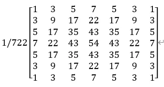
• For the original image \(f(x,y)\), apply Gaussian blur to obtain the smoothed image \(\overline{f(x,y)}\).
• Take the difference between the original image and the smoothed image to obtain the mask \(g_{mask}(x,y)=f(x,y)-\overline{f(x,y)}\).
• Add the original image and k times the mask to obtain the enhanced image \(g(x,y)=f(x,y)+k*g_{mask}(x,y)\).
• Generally, the value of k is set to 1 for image enhancement. If k is greater than 1, it is a high-boost image.

The image processing effect of this algorithm is as follows:

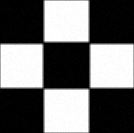
From left to right: original image, obtained mask (normalized to 0-255), enhanced image

From the results in the above figure, it can be seen that the mask image has high brightness at the edges and low brightness elsewhere. After overlaying with the original image, the brightness of the original image's edges becomes larger. In this case, the method used here is to normalize the overlaid image as a whole and then multiply it by 255 to obtain an integer value. Because the brightness of the original image's edges is large after overlaying with the mask, the bright parts in the original image become darker after normalization. If another method is used, such as treating values greater than 255 as 255 and values less than 0 as 0, it can effectively solve this problem, but the edges of the image will not be as obvious as the previous method. The specific method to be used depends on the actual situation.

Sobel Operator

The Sobel operator is often used for edge extraction in images. It uses the first-order derivative of the image to extract edges, which is denoted as \(\nabla f\).

We know that the gradient of a binary function consists of the directional derivatives in the x and y directions. The Sobel operator is the same, with two operators for the x and y directions, respectively, as follows: \[ \begin{bmatrix}-1&0&1\\-1&0&2\\-1&0&1\end{bmatrix} ~~~~~~~~~~\begin{bmatrix}-1&-2&-1\\0&0&0\\1&2&1\end{bmatrix} \]

• Convolve the image with the above two operators separately to obtain the x-direction and y-direction edges \(G_x\) and \(G_y\).
• The first-order derivative of the image \(G\) can be calculated using \(G_x\) and \(G_y\), which is \(G=\sqrt{G_x^2+G_y^2}\). Sometimes, for fast calculation, \(G=|G_x|+|G_y|\) or \(G=max\{|G_x|,|G_y|\}\) can be used.
• Normalize G to the range of 0-255 to obtain the Sobel edges of the image.

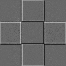
From left to right: original image, x-direction edges, y-direction edges, Sobel edges

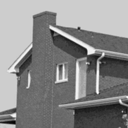
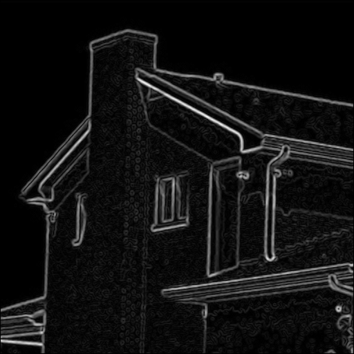
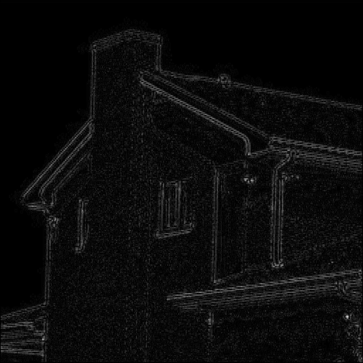
The Sobel operator performs well in extracting obvious edges in images and also performs well in extracting detailed edges in images. This can be illustrated by the processing results of another image:

It can be seen that even the small edge contours on the chimney are well represented by the edges extracted by the Sobel operator.

Laplacian Operator

\[ [f(x+1)-f(x)]-[f(x)-f(x-1)]=f(x+1)+f(x-1)-2f(x) \] From this, the Laplacian operator can be derived as: \[ \begin{bmatrix}0&1&0\\1&-4&1\\0&1&0\end{bmatrix} \] Sometimes, the second-order derivative in the diagonal direction is also added, and the operator becomes: \[ \begin{bmatrix}1&1&1\\1&-8&1\\1&1&1\end{bmatrix} \] In practice, the following two operators are often used: \[ \begin{bmatrix}0&-1&0\\-1&4&-1\\0&-1&0\end{bmatrix} \begin{bmatrix}-1&-1&-1\\-1&8&-1\\-1&-1&-1\end{bmatrix} \]

Assuming that the extracted image edges are \(L(x,y)\), the algorithm for image enhancement is \(g(x,y)=f(x,y)+c*L(x,y)\)

If the above two operators are used to extract the edges, c=-1; if the following two operators are used, c=1.

The image edge information extracted using the Laplacian operator is as follows:

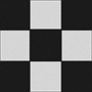
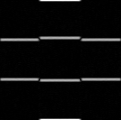
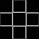
From left to right: original image, Laplacian edges without diagonal, Laplacian edges with diagonal

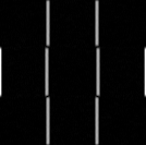
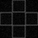
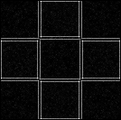
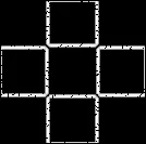
The edges extracted by the Laplacian operator have two edge lines at each edge, which is determined by the properties of its second-order derivative. Compared with the edges extracted by the Sobel operator, the Laplacian edges are more detailed and capture the "edges of edges". This can be seen more clearly from the comparison in the following figure:

The left side is the result of the Sobel operator, and the right side is the result of the Laplacian operator

For slightly more complex images, the edges extracted by the Laplacian operator are too detailed, making it difficult to see many areas clearly, which poses some difficulties for human visual perception. However, in some image recognition fields, such as using satellite images to identify ground vehicles, the vehicles on the ground are often small color blocks, and the Laplacian operator can well outline the edge contours and some details inside these vehicles. The Sobel operator is not as effective in capturing these internal details. At the same time, the property of "edges of edges" makes the edges extracted by the Laplacian operator suitable for image enhancement.

Canny Algorithm

The Canny algorithm is an optimization of the Sobel edge extraction. The Sobel operator represents all edges in the final image, regardless of their strength. This results in many invalid edges being extracted and displayed in the resulting image. The basic idea of the Canny algorithm is to filter out these edge information and only keep the pixels that are most likely to be edges. The implementation method is as follows:

• Similar to the Sobel operator, calculate \(G_x\) and \(G_y\).
• Calculate the weight \(weight=\sqrt{G_x^2+G_y^2}\) and the angle \(angle=atan\frac{G_y}{G_x}\) for each pixel based on \(G_x\) and \(G_y\).
• Discretize the angle to the nearest multiple of \(45^o\).
• For each pixel \((x,y)\) in the image, compare its weight \(weight(x,y)\) with the weights of the two pixels in the \(angle(x,y)\) direction and \(-angle(x,y)\) direction. If the weight of the pixel is not the largest, set it to 0.
• Double threshold detection: set upper and lower thresholds for the brightness of the edges, and perform another filtering on the edges of the image. Finally, normalize the edge information to the range of 0-255. The thresholds can be manually set.

From left to right: original image, edges without double threshold detection, edges with lower threshold of 150, edges with lower threshold of 200

Appendix

References

[1] Rafael C. Gonzalez and Richard E. Woods, "Digital Image Processing", 3rd Edition, Beijing: Publishing House of Electronics Industry, 2017.

[2] Brook_icv, "Image Processing Basics (4): Gaussian Filter Detailed Explanation" [Online]. Available: https://www.cnblogs.com/wangguchangqing/p/6407717.html#autoid-4-1-0

[3] Naughty Stone 7788121, "Image Edge Detection: Canny Operator, Prewitt Operator, and Sobel Operator" [Online]. Available: https://www.jianshu.com/p/bed4ffe996a1

Source Code

1
2
3
4
5
6
7
8
9
10
11
12
13
14
15
16
17
18
19
20
21
22
23
24
25
26
27
28
29
30
31
32
33
34
35
36
37
38
39
40
41
42
43
44
45
46
47
48
49
50
51
52
53
54
55
56
57
58
59
60
61
62
63
64
65
66
67
68
69
70
71
72
73
74
75
76
77
78
79
80
81
82
83
84
85
86
87
88
89
90
91
92
93
94
95
96
97
98
99
100
101
102
103
104
105
106
107
108
109
110
111
112
113
114
115
116
117
118
119
120
121
122
123
124
125
126
127
128
129
130
131
132
133
134
135
136
137
138
139
140
141
142
143
144
145
146
147
148
149
150
151
152
153
154

import cv2 as cv
import numpy as np
import math

sigma=1.5   # Parameter of the Gaussian filter

def add_zeros(img,edge):    # Add zeros to the edges of the image
    shape=img.shape
    temp=np.zeros((shape[0]+2*edge,shape[1]+2*edge))
    for i in range(shape[0]):
        for j in range(shape[1]):
            temp[i+edge][j+edge]=img[i][j][0]
    return temp

def f(x,y):     # Define the 2D Gaussian distribution function
    return 1/(math.pi*sigma**2)*math.exp(-(x**2+y**2)/(2*sigma**2))

def gauss(n):   # Generate an n*n Gaussian filter
    mid=n//2
    filt=np.zeros((n,n))
    for i in range(n):
        for j in range(n):
            filt[i][j]=f(i-mid,j-mid)/f(-mid,-mid)
    return filt.astype(np.uint8)

def gauss_filter(img,n):    # Apply n*n convolutional blocks of Gaussian filtering to the image
    filt=gauss(n)
    con=1/np.sum(filt)
    shape=img.shape
    temp=add_zeros(img,n//2)
    result=np.zeros((shape[0],shape[1],1))
    for i in range(shape[0]):
        for j in range(shape[1]):
            tmp=0
            for k in range(n):
                for l in range(n):
                    tmp+=filt[k][l]*temp[i+k][j+l]
            result[i][j][0]=con*tmp
    return result.astype(np.uint8)

def unsharp_mask(img,n,is_mask=0):        # Unsharp mask using n*n Gaussian blur, return the mask if is_mask=1
    shape=img.shape
    new_img=np.zeros((shape[0],shape[1],1))
    for i in range(shape[0]):
        for j in range(shape[1]):
            new_img[i][j][0]=img[i][j][0]
    mask=new_img-gauss_filter(img,n)
    for i in range(shape[0]):
        for j in range(shape[1]):
            if i==0 or j==0 or i==shape[0]-1 or j==shape[1]-1:
                mask[i][j][0]=0
    result=new_img+mask
    result=result-np.min(result)
    result=result/np.max(result)*255
    mask=mask-np.min(mask)
    mask=mask/np.max(mask)*255
    if is_mask:
        return mask.astype(np.uint8)
    return result.astype(np.uint8)

sobelx=[[-1,0,1],[-2,0,2],[-1,0,1]]
sobely=[[-1,-2,-1],[0,0,0],[1,2,1]]
laplace4=[[0,-1,0],[-1,4,-1],[0,-1,0]]
laplace8=[[-1,-1,-1],[-1,8,-1],[-1,-1,-1]]

def filt_3(img,filt):          # Arbitrary 3*3 filter (image, operator)
    shape=img.shape
    temp=add_zeros(img,1)
    result=np.zeros((shape[0],shape[1],1))
    for i in range(shape[0]):
        for j in range(shape[1]):
            tmp=0
            for k in range(3):
                for l in range(3):
                    tmp+=filt[k][l]*temp[i+k][j+l]
            result[i][j][0]=tmp
    return result

def laplace_edge(img,filt): # Laplacian edges after normalization
    tmp=filt_3(img,filt)
    tmp=tmp-np.min(tmp)
    shape=tmp.shape
    for i in range(shape[0]):
        for j in range (shape[1]):
            if i==0 or j==0 or i==shape[0]-1 or j==shape[1]-1:
                tmp[i][j][0]=0
    tmp=tmp/np.max(tmp)*255
    return tmp.astype(np.uint8)

def laplace(img,filt):  # Overlay of the original image and the Laplacian edges
    tmp=filt_3(img,filt)
    shape=img.shape
    result=np.zeros((shape[0],shape[1]))
    for i in range(shape[0]):
        for j in range(shape[1]):
            result[i][j]=tmp[i][j][0]+img[i][j][0]
            if i==0 or j==0 or i==shape[0]-1 or j==shape[1]-1:
                result[i][j]=0
    result-=np.min(result)
    result=result/np.max(result)*255
    return result.astype(np.uint8)

def sobel(img):     # Extract Sobel edges of the image
    shape=img.shape
    sobx=filt_3(img,sobelx)
    soby=filt_3(img,sobely)
    result=np.zeros((shape[0],shape[1]))
    for i in range(shape[0]):
        for j in range(shape[1]):
            if i==0 or j==0 or i==shape[0]-1 or j==shape[1]-1:
                result[i][j]=0
            else:
                result[i][j]=math.sqrt(sobx[i][j][0]**2+soby[i][j][0]**2)
    result=result/np.max(result)*255
    return result.astype(np.uint8)

def canny(img,n=3):     # Extract image edges using the Canny algorithm (blur operation using an n*n Gaussian filter)
    de=[[1,0,-1,0],[1,1,-1,-1],[0,1,0,-1],[-1,1,1,-1]]
    shape=img.shape
    tmp=gauss_filter(img,n)
    sobx=filt_3(tmp,sobelx)
    soby=filt_3(tmp,sobely)
    weight,angle,result=np.zeros((shape[0],shape[1])),np.zeros((shape[0],shape[1])),np.zeros((shape[0],shape[1]))
    angle=angle.astype(np.int)
    for i in range(shape[0]):
        for j in range(shape[1]):
            weight[i][j]=math.sqrt(sobx[i][j][0]**2+soby[i][j][0]**2)
            if sobx[i][j][0]:
                angle[i][j]=round((math.atan(soby[i][j][0]/sobx[i][j][0])/(math.pi/4)-0.5))%4
    for i in range(shape[0]-2):
        for j in range(shape[1]-2):
            tmp_i,tmp_j=i+1,j+1
            if weight[tmp_i][tmp_j]<=weight[tmp_i+de[angle[tmp_i][tmp_j]][0]][tmp_j+de[angle[tmp_i][tmp_j]][1]] and weight[tmp_i][tmp_j]<=weight[tmp_i+de[angle[tmp_i][tmp_j]][2]][tmp_j+de[angle[tmp_i][tmp_j]][3]]:
                result[tmp_i][tmp_j]=0
            else:
                result[tmp_i][tmp_j]=weight[tmp_i][tmp_j]
    result=result/np.max(result)*255
    mean=np.mean(img)
    for i in range(shape[0]):
        for j in range(shape[1]):
            if result[i][j]<100:
                result[i][j]=0
    return result.astype(np.uint8)


filename=["test3_corrupt.pgm","test4.tif"]
for i in filename:
    img=cv.imread(i)
    cv.imwrite(i+"_mask.bmp",unsharp_mask(img,3,1))
    cv.imwrite(i+"_unsharp_mask.bmp",unsharp_mask(img,3))
    cv.imwrite(i+"_sobel.bmp",sobel(img))
    cv.imwrite(i+"_canny.bmp",canny(img,3))
    cv.imwrite(i+"laplace4_edge.bmp",laplace_edge(img,laplace4))
    cv.imwrite(i+"laplace8_edge.bmp",laplace_edge(img,laplace8))

低通滤波器在我们的日常生活中很有用，图像模糊，图像去噪以及图像识别都需要低通滤波器的处理。低通滤波即滤除图像中的高频部分（变化很快的部分），留下低频部分（变化不明显得到部分）。滤波器的实现有空域和频域两种：空域滤波器是直接在空间图像上进行操作，图像矩阵和滤波器算子进行卷积得到滤波后的输出；频域滤波器是将图像经过傅里叶变换到频域上再与滤波器做乘法得到输出。

Low-pass filters are very useful in our daily lives. Image blurring, image denoising, and image recognition all require the use of low-pass filters. Low-pass filtering means removing the high-frequency components (rapidly changing parts) from an image and leaving the low-frequency components (parts with less noticeable changes). There are two implementations of filters: spatial domain and frequency domain. Spatial domain filters operate directly on the spatial image, convolving the image matrix with the filter kernel to obtain the filtered output. Frequency domain filters transform the image to the frequency domain using the Fourier transform and then multiply it with the filter to obtain the output.

This article mainly introduces spatial domain low-pass filters and their implementations.

Commonly used spatial domain filters include average filtering, median filtering, and Gaussian filtering. Here, we mainly introduce median filtering and Gaussian filtering.

Median Filtering

As the name suggests, median filtering is a filter based on statistical methods. The specific implementation method is as follows: for an n*n median filter, the pixel value of the output image at (x, y) is equal to the median of all pixel values in the n*n image area centered at (x, y) in the input image.

The size of the filter can be selected according to different needs.

The effect of the median filter is as follows:

The original image, 3*3 median filter, 5*5 median filter, and 7*7 median filter, respectively.

Original Image

3*3 Median Filter

5*5 Median Filter

7*7 Median Filter

The original image contains a lot of irregularly distributed noise, some of which are salt noise, but most of them are sudden impulse noise. When using a 3*3 median filter, the salt noise has been removed well, but the impulse noise is still obvious. When using a 5*5 median filter, the situation of impulse noise has been greatly improved. The 7*7 filter almost completely removes the noise, but the image is also severely blurred.

Gaussian Filtering

Gaussian filtering is a commonly used blurring method in some image processing software. It is generated by the two-dimensional normal distribution function: \(p(x,y)=\frac1{2\pi\sigma^2}e^{-\frac{x^2+y^2}{2\sigma^2}}\). The specific steps are as follows:

• To generate an n*n Gaussian filter, set the center of the n-order simulation to (0,0) and generate the coordinates of other positions in the matrix.
• Substitute the coordinates of each position in the n*n matrix into the two-dimensional normal distribution function to obtain the value of each position.
• Scale the values in the matrix based on the value of 1 in the upper left corner of the matrix.
• Round the matrix to obtain the n*n Gaussian filter.

The function for generating a Gaussian filter is as follows:

1 2 3 4 5 6 7 8 9 10 11 12

import numpy as np sigma=1.5 # Parameter of the Gaussian filter def f(x,y): # Define the two-dimensional normal distribution function return 1/(math.pi*sigma**2)*math.exp(-(x**2+y**2)/(2*sigma**2)) def gauss(n): # Generate an n*n Gaussian filter mid=n//2 filt=np.zeros((n,n)) for i in range(n): for j in range(n): filt[i][j]=f(i-mid,j-mid)/f(-mid,-mid) return filt.astype(np.uint8)

The Gaussian filters of size 3*3, 5*5, and 7*7 are as follows:

Their images in the two-dimensional coordinate system are as follows:

After obtaining the operator of the Gaussian filter, convolve it with the input image to obtain the result of the Gaussian filter.

The effect is as follows:

The original image, 3*3, 5*5, and 7*7 Gaussian filtering results:

Original Image

3*3 Gaussian

5*5 Gaussian

7*7 Gaussian

Gaussian blur is more effective in removing salt noise in the image, but it is more difficult to remove impulse noise. The 7*7 Gaussian filter still cannot remove the impulse noise in the image. On the other hand, compared with Gaussian blur, Gaussian blur retains more information of the image and preserves more details.

Appendix

References

[1] Digital Image Processing, Third Edition / (Rafael C. Gonzalez), translated by Ruan Qiuqi, et al. - Beijing: Electronic Industry Press, 2017.5

[2] Brook_icv. Basic Image Processing (4): Detailed Explanation of Gaussian Filters [G/OL]. Blog Garden: 2017-02-16 [2020-03-23]. https://www.cnblogs.com/wangguchangqing/p/6407717.html#autoid-4-1-0

[3] Yu Ni Xin An. Methods for Calculating Mean, Median, and Mode in Numpy [G/OL]. Blog Garden: 2018-11-04 [2020-03-23]. https://www.cnblogs.com/lijinze-tsinghua/p/9905882.html

Source Code

1
2
3
4
5
6
7
8
9
10
11
12
13
14
15
16
17
18
19
20
21
22
23
24
25
26
27
28
29
30
31
32
33
34
35
36
37
38
39
40
41
42
43
44
45
46
47
48
49
50
51
52
53
54
55
56
57
58
59
60

import cv2 as cv
import numpy as np
import math
img=cv.imread("test1.pgm")

sigma=1.5   # Parameter of the Gaussian filter
def f(x,y):     # Define the two-dimensional normal distribution function
    return 1/(math.pi*sigma**2)*math.exp(-(x**2+y**2)/(2*sigma**2))

def gauss(n):   # Generate an n*n Gaussian filter
    mid=n//2
    filt=np.zeros((n,n))
    for i in range(n):
        for j in range(n):
            filt[i][j]=f(i-mid,j-mid)/f(-mid,-mid)
    return filt.astype(np.uint8)

def gauss_filter(img,n):    # Perform Gaussian filtering on the image img with an n*n convolution block
    filt=gauss(n)
    con=1/np.sum(filt)
    shape=img.shape
    mid=n//2
    temp=np.zeros((shape[0]+n-1,shape[1]+n-1))   # Pad the edges with zeros
    for i in range(shape[0]):
        for j in range(shape[1]):
            temp[i+mid][j+mid]=img[i][j][0]
    result=np.zeros((shape[0],shape[1]))
    for i in range(shape[0]):
        for j in range(shape[1]):
            tmp=0
            for k in range(n):
                for l in range(n):
                    tmp+=filt[k][l]*temp[i+k][j+l]
            result[i][j]=con*tmp
    return result.astype(np.uint8)

def center_filter(img, n):  # Perform low-pass filtering on the image using an n*n median filter
    mid=n//2
    shape=img.shape
    temp=np.zeros((shape[0]+n-1,shape[1]+n-1))
    for i in range(shape[0]):
        for j in range(shape[1]):
            temp[i+mid][j+mid]=img[i][j][0]
    result=np.zeros((shape[0],shape[1]))
    tmp=np.zeros(n*n)
    for i in range (shape[0]):
        for j in range(shape[1]):
            for k in range(n):
                for l in range(n):
                    tmp[k*n+l]=temp[i+k][j+l]
            result[i][j]=np.median(tmp)
    return result.astype(np.uint8)

filename=["test1.pgm","test2.tif"]
size=[3,5,7]
for i in filename:
    img=cv.imread(i)
    for j in size:
        cv.imwrite(i+'gauss-'+str(j)+'.bmp',gauss_filter(img,j))
        cv.imwrite(i+'center-'+str(j)+'.bmp',center_filter(img,j))

总体设计思路

视频的播放实际上就是一系列的图片按照一定的顺序，以一定的时间间隔连续播放所产生的视觉效果。因此，使用单片机驱动LCD去播放视频实际上就是让单片机以一定的时间间隔向LCD的缓存推送图片，让其不断刷新屏幕去切换图片即可。在文章的最后我放入了这个项目的源工程文件供大家参考。

Overall Design Concept

The playback of a video essentially involves a sequence of images displayed in a specific order at regular time intervals, creating a visual effect. Therefore, driving an LCD to play a video with a microcontroller involves pushing images to the LCD's buffer at certain intervals, continuously refreshing the screen to switch images. At the end of the article, I've included the source project files for reference.

在数字图像处理中，直方图均衡是调整图像亮度，对比度，图像增晰等操作中常用的做法。对于图像中各个不同的颜色进行直方图统计，采取统计数据对于颜色进行重新映射，从而达到调整对比度，图像增晰的目的。

In digital image processing, histogram equalization is a common practice used to adjust brightness, contrast, and image sharpening. It involves statistical analysis of the histogram of different colors in an image, followed by remapping the colors based on this analysis to achieve the desired adjustments in contrast and sharpness.

1. Histogram of Digital Images

A histogram refers to the statistical analysis of all the pixel colors in an entire image, presenting the statistical data of different colors in the form of a histogram.

For example, consider the following two images:

Their corresponding histograms are:

From these figures, it can be observed that an image with high contrast has a wider distribution of colors, while an image with low contrast has colors concentrated in a specific region. In the second image, the pixel values are concentrated on a single color, resulting in image blurring.

Using image histograms, the color distribution of an image can be clearly understood, providing guidance on how to enhance images and improve contrast.

2. Histogram Equalization

Histogram equalization, as the name suggests, aims to equalize the color distribution in an image histogram. Specifically, it redistributes colors that were previously too concentrated in the histogram, spreading them out to occupy the appropriate pixel values. The specific method is as follows (using 3-bit 8-color as an example):

Consider a 64x64 pixel image (M=64, N=64, MN=4096) with 3 bits (L=8) representing colors, ranging from [0,L-1], i.e., [0,7]. By performing statistical analysis on the pixel values of the entire image, we obtain the following statistical data:

图像配准即对于内容大致相同，但在角度，大小或是其他几何位置上有所偏差的两张或几张图像进行坐标变换。使得这些图像矫正到同一规整的大小，角度，坐标上。

图像配准对于图像拼接，制作全景图像，进行环境识别等方面有很大的用处。其原理简单，使用矩阵运算转换速度也很快，在选取映射点合适的情况下，配准效果很好。具体的转化方法如下：