XJTU System Optimization and Scheduling Midterm Report
Midterm Report
西安交通大学《系统优化与调度》课程中期报告

Problem
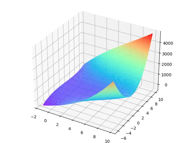
\[ min\ \ x_1^3+x_2^3-2x_1^2x_2+5x_1x_2^2+10x_1x_2+7x_1-x_2\\ s.t.\left\{ \begin{array}{**lr**} -x_1+x_2\leq0\\ -2x_1-5x_2-10\leq0\\ x_1-100\leq 0 \end{array} \right. \]
The graph of the object function is shown below:
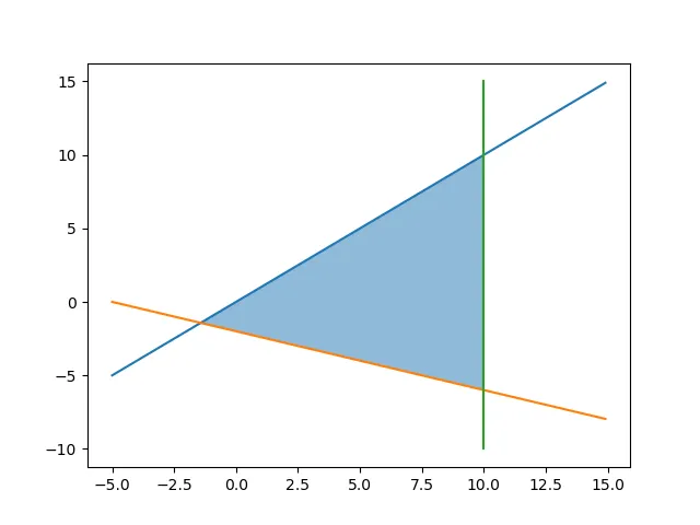
The feasible region by the constraint is shown blow:
Method
For this problem, we can see that the feasible region is a convex set, and the object function is not convex. Considering the feasible region, the constraint works only when searching out the boundary. Using projection method could let the searched point outing the boundary move to the boundary. So the method I using is below:
- choose the start point \(x^0\)
- replace point with the projection\([x^0]^+\)
- get the projection of next direction point \(\bar x_k=[x^k-\nabla f(x^k)]^+\)
- get the search direction \(d^k=\bar x^k-x^k\)
- calculate the next point \(x^{k+1}=x^k+\alpha^kd^k\)
- if the terminal condition is satisficed, stop the search and output the result, else go to the step 3
In this project, I choose Armjio rule to control the step size.
The parameters of the method is following: \[ s=1\ \ \beta=0.5\ \ \sigma=1e-5 \]
Solution
Considering the floating error of computers, stipulate \(a=b\) when \(|a-b|<\varepsilon\), and \(a=0\) if \(|a|<\varepsilon\). In this project, \(\varepsilon=1e-19\).
choose the start point (0,0), we could get the following answer:
| \(x^k\) | \(f(x^k)\) | \(\alpha^k\) | \(d^k\) | |
|---|---|---|---|---|
| 1 | (0,0) | 0 | 1 | (-1.42857,-1.42857) |
| 2 | (-1.42857,-1.42857) | -2.74052 | 1 | (1.71358,-0.68543) |
| 3 | (0.28501,-2.11400) | -4.62839 | 0.5 | (-1.71358,0.68543) |
| 4 | (-0.57178,-1.77129) | -5.65909 | 0.25 | (2.55462,-1.02185) |
| 5 | (0.06688,-2.02675) | -5.79388 | 0.25 | (-1.49545,0.59818) |
| 6 | (-0.30699,-1.87721) | -6.20808 | 0.125 | (0.86671,-0.34668) |
| 7 | (-0.19865,-1.92054) | -6.25856 | 0.125 | (-0.08902,0.03561) |
| 8 | (-0.20977,-1.91609) | -6.25903 | 0.125 | (0.01624,-0.00649) |
| 9 | (-0.20775,-1.91690) | -6.25904 | 0.125 | (-0.00284,0.00114) |
| 10 | (-0.20810,-1.91676) | -6.25904 | 0.125 | (0.00050,-0.00020) |
| 11 | (-0.20804,-1.91679) | -6.25904 | 0.125 | (-0.00009,0.00004) |
| 12 | (-0.20805,-1.91678) | -6.25904 | 0.125 | (0.00002,-0.00001) |
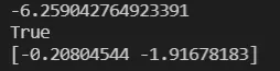
The final result is \(x^*=[-0.20805, -1.91678],f(x^*)=-6.25904\).
same as the result solved by the python package
scipy.optimize.minimize:
Change the start point to (5,-8), and the answer following:
| \(x^k\) | \(f(x^k)\) | \(\alpha^k\) | \(d^k\) | |
|---|---|---|---|---|
| 1 | (6.37931,-4.55172) | 955.45385 | 1 | (-7.80788,3.12315) |
| 2 | (-1.42857,-1.42857) | -2.74052 | 1 | (1.71358,-0.68543) |
| 3 | (0.28501,-2.11400) | -4.62839 | 0.5 | (-1.71358,0.68543) |
| 4 | (-0.57178,-1.77129) | -5.65909 | 0.25 | (2.55462,-1.02185) |
| 5 | (0.06688,-2.02675) | -5.79388 | 0.25 | (-1.49545,0.59818) |
| 6 | (-0.30699,-1.87721) | -6.20808 | 0.125 | (0.86671,-0.34668) |
| 7 | (-0.19865,-1.92054) | -6.25856 | 0.125 | (-0.08902,0.03561) |
| 8 | (-0.20977,-1.91609) | -6.25903 | 0.125 | (0.01624,-0.00649) |
| 9 | (-0.20775,-1.91690) | -6.25904 | 0.125 | (-0.00284,0.00114) |
| 10 | (-0.20810,-1.91676) | -6.25904 | 0.125 | (0.00050,-0.00020) |
| 11 | (-0.20804,-1.91679) | -6.25904 | 0.125 | (-0.00009,0.00004) |
| 12 | (-0.20805,-1.91678) | -6.25904 | 0.125 | (0.00002,-0.00001) |
We can see that the searching point went to the boundary quickly, and then the trajectory of the searching is same as ahead.
Appendix
1 | language: python |
The source code is following:
1 | from math import sqrt |