本文主要对于交叉熵的手动计算和PyTorch中的CrossEntropyLoss模块计算结果不一致的问题展开讨论，查阅了PyTorch的官方文档，最终发现是CrossEntropyLoss在计算交叉熵之前会对输入的概率分布进行一次SoftMax操作导致的。

This article mainly discusses the inconsistency between the manual calculation of cross-entropy and the results obtained by the CrossEntropyLoss module in PyTorch. After consulting the official documentation of PyTorch, it was found that the inconsistency was caused by the SoftMax operation performed by CrossEntropyLoss on the input probability distribution before calculating the cross-entropy.

In reinforcement learning, the loss function commonly used in policy learning is \(l=-\ln\pi_\theta(a|s)\cdot g\), where \(\pi_\theta\) is a probability distribution over actions given state \(s\), and \(a\) is the action selected in state \(s\). Therefore, we have:

\[ -\ln\pi_\theta(a|s) = -\sum_{a'\in A}p(a')\cdot \ln q(a') \]

\[ p(a') = \left\{ \begin{array}{lr} 1 &&& a'=a\\ 0 &&& otherwise \end{array} \right. \]

\[ q(a') = \pi_\theta(a'|s) \]

Thus, this loss function is transformed into the calculation of cross-entropy between two probability distributions. Therefore, we can use the built-in torch.nn.functional.cross_entropy function (referred to as the F.cross_entropy function below) in PyTorch to calculate the loss function. However, in practice, it was found that the results calculated using this function were inconsistent with the results calculated manually, which led to a series of investigations.

Firstly, we used Python to manually calculate the cross-entropy of two sets of data and the cross-entropy calculated using the F.cross_entropy function, as shown in the code below:

1
2
3
4
5
6
7
8
9
10
11
12
13

import torch
from torch.nn import functional as F

x = torch.FloatTensor([[0.4, 0.6],
                       [0.7, 0.3]])
y = torch.LongTensor([0, 1])

loss_1 = -torch.log(x.gather(1, y.view(-1,1)))
loss_2 = F.cross_entropy(x, y, reduction = "none")

print("Manually calculated cross-entropy:\n{}".format(loss_1.squeeze(1)))
print()
print("CrossEntropyLoss calculated cross-entropy:\n{}".format(loss_2))

The results of the above code are as follows:

1
2
3
4
5

Manually calculated cross-entropy:
tensor([0.9163, 1.2040])

CrossEntropyLoss calculated cross-entropy:
tensor([0.7981, 0.9130])

From the results, it can be seen that the two calculation results are not consistent. Therefore, we consulted the official documentation of PyTorch to understand the implementation of F.cross_entropy.

The description of the F.cross_entropy function in the documentation does not include the specific calculation process, only explaining the correspondence between the input data and the output result dimensions ¹. However, there is a sentence in the introduction of this function:

See CrossEntropyLoss for details.

So we turned to the documentation of CrossEntropyLoss ² and finally found the calculation process of cross-entropy in PyTorch:

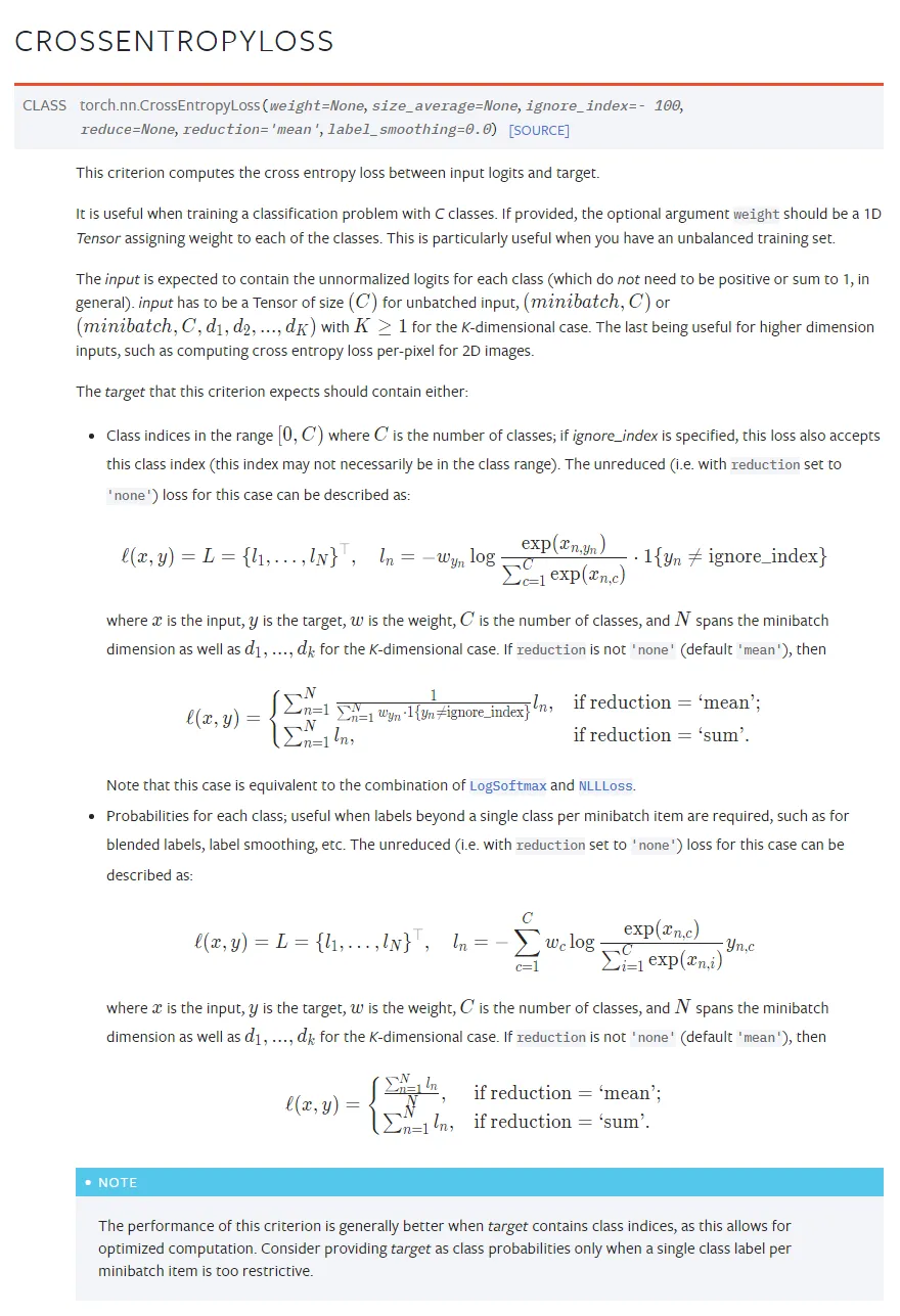
It can be seen that the official documentation on the calculation of cross-entropy is very clear. In summary, the F.cross_entropy function requires at least two parameters, one is the predicted probability distribution, and the other is the index of the target true class. The important point is that the F.cross_entropy function does not require the input probability distribution to sum to 1 or each item to be greater than 0. This is because the function performs a SoftMax operation on the input probability distribution before calculating the cross-entropy.

Performing the SoftMax operation before calculating the cross-entropy improves the tolerance of the input, but if the SoftMax operation has been performed before the output is constructed in the neural network, it will cause the calculation of loss to be distorted, that is, the calculation results of the previous section are inconsistent.

According to the official documentation of PyTorch, if we add a SoftMax operation to the manual calculation of cross-entropy, we can get the same calculation result as the F.cross_entropy function. The following code is used to verify this:

1
2
3
4
5
6
7
8
9
10
11
12
13

import torch
from torch.nn import functional as F

x = torch.FloatTensor([[0.4, 0.6],
                       [0.7, 0.3]])
y = torch.LongTensor([0, 1])

loss_1 = -torch.log(F.softmax(x, dim=-1).gather(1, y.view(-1,1)))
loss_2 = F.cross_entropy(x, y, reduction = "none")

print("Manually calculated cross-entropy:\n{}".format(loss_1.squeeze(1)))
print()
print("CrossEntropyLoss calculated cross-entropy:\n{}".format(loss_2))

The output of the above code is as follows:

1
2
3
4
5

Manually calculated cross-entropy:
tensor([0.7981, 0.9130])

CrossEntropyLoss calculated cross-entropy:
tensor([0.7981, 0.9130])

Reference

最近在逐一复现RL算法过程中，策略梯度算法的收敛性一直有问题。经过一番探究和对比实验，学习了网上和书本上的很多实验代码之后，发现了代码实现中的一个小问题，即Policy Gradient在计算最终loss时求平均和求和对于网络训练的影响，本文将对此进行展开讨论。

先说结论：

在进行策略梯度下降优化策略时，可以对每个动作的loss逐一（for操作）进行反向传播后进行梯度下降，也可以对每个动作的loss求和（sum操作）之后进行反向传播后梯度下降，但尽量避免对所有动作的loss求平均（mean操作）之后进行反向传播后梯度下降，这会导致收敛速度较慢，甚至无法收敛。

具体的论证和实验过程见下文。

Zotero 是一款非常好用的开源文献管理软件，在对比了Endnote，Mendeley，Zotero之后最终我选择了Zotero作为我自己的文献管理软件，选择其的主要原因有：

• 支持webdav同步文献记录及pdf附件
• 丰富的扩展插件
• 支持markdown笔记

本文主要介绍部分常用的Zotero插件，并附上其下载链接，同时谈谈使用感受。顺序按照我个人认为的好用程度排序。

Zotero is a very useful open-source reference management software. After comparing Endnote, Mendeley, and Zotero, I ultimately chose Zotero as my own reference management software for the following reasons:

• Support for webdav synchronization of reference records and PDF attachments
• Rich extension plugins
• Support for markdown notes

This article mainly introduces some commonly used Zotero plugins, along with their download links, and discusses my experience using them. The order is based on what I personally consider to be the most useful.

本文围绕自由落体运动的估计，进行了线性滤波和非线性滤波的实验。下面这张图是源自西安交通大学蔡远利教授的《随即滤波与控制》课程。 该课程主要围绕估计，平滑与预测三方面讲解各类滤波方法。

This article presents experiments on linear filtering and nonlinear filtering for estimating the free fall motion. The following figure is from Professor Cai Yuanli's course "Random Filtering and Control" at Xi'an Jiaotong University. The course mainly discusses various filtering methods related to estimation, smoothing, and prediction.

智能体对战目标检测

手动标注数据集及视频分割程序下载见文章末。

Intelligent Agent for Target Detection in Game Battles

Manual annotation dataset and video segmentation program download can be found at the end of the article.