爬取B站所有番剧数据并进行数据分析

简介

Bilibili(以下简称B站)中有大量的番剧版权,截止目前一共有3161部。每一部番剧都可以找到它的播放量追番量弹幕数量等播放数据,除此之外,每部番剧还有其相应的标签(如“漫画改”,“热血”,“搞笑”)。本项目旨在分析番剧播放数据与番剧标签之间的关系,同时也是一项数据分析的大作业,采用APriori频繁项集挖掘进行分析。

GitHub地址:https://github.com/KezhiAdore/BilibiliAnimeData_Analysis

码云地址:https://gitee.com/KezhiAdore/BilibiliAnimeData_Analysis

数据收集

首先要获取到需要的所有数据,即B站所有番剧播放信息和标签信息。使用爬虫对数据进行爬取,这里使用的是python的scrapy编写爬虫对数据进行爬取。

页面分析

首先来到番剧索引页面

从该页面点击某部番剧进入其详情页

可以看到该页面中就有需要的番剧播放数据以及番剧的标签。

对该页面的HTML进行分析得到数据所在的xpath路径,以tag为例:

所有数据对应的xpath路径分别为:

1
2
3
4
标签: //span[@class="media-tag"]
总播放: //span[@class="media-info-count-item media-info-count-item-play"]/em
追番人数: //span[@class="media-info-count-item media-info-count-item-fans"]/em
弹幕总数: //span[@class="media-info-count-item media-info-count-item-review"]/em

那么到现在来说循环进入所有的番剧列表页,从该页面进入番剧详情页并对每个番剧详情页进行解析,数据保存就可以了,但此时出现了问题。对番剧列表页进行爬取之后的网页数据相应的地方为:

直接对该页面进行访问无法获取到详细的番剧列表信息。由此,转而对页面接受到的文件进行分析,找到了该页面获取的番剧列表信息文件。

访问该url得到的信息为:

对该api网址进行分析,易得page=1控制着页数信息,通过改变该信息即可访问不同的番剧列表页面。

1
https://api.bilibili.com/pgc/season/index/result?season_version=-1&area=-1&is_finish=-1&copyright=-1&season_status=-1&season_month=-1&year=-1&style_id=-1&order=3&st=1&sort=0&page=1&season_type=1&pagesize=20&type=1

该页面获取到的信息为json文件,内含信息格式如下:

与番剧详情页的网址https://www.bilibili.com/bangumi/media/md22718131进行比对可以发现,json文件中的media_id数据即为每个番剧详情页的标识,由此,爬取信息的逻辑基本建立了。

  1. 访问起始api页面(page=1),对其内容进行解析,获取到该页所有番剧的media_id
  2. 利用media_id构建访问番剧详情页的链接,爬取该页面进行解析,得到一个番剧的数据
  3. 访问下一个api页面,再次进行上述操作。

爬虫构建

首先初始化爬虫

1
2
scrapy startproject anime_data
scrapy genspider anime ""

文件树如下

打开items.py,建立需要保存的数据对象

1
2
3
4
5
6
7
8
9
10
import scrapy

class AnimeDataItem(scrapy.Item):
# define the fields for your item here like:
name = scrapy.Field() #番剧名称
play=scrapy.Field() #总播放量
fllow=scrapy.Field() #追番人数
barrage=scrapy.Field() #弹幕数量
tags=scrapy.Field() #番剧标签,列表形式
pass

再打开刚建立的anime.py,访问页面,解析以及数据保存的代码如下

1
2
3
4
5
6
7
8
9
10
11
12
13
14
15
16
17
18
19
20
21
22
23
24
25
26
27
28
29
30
31
32
33
34
35
36
37
38
import scrapy
import json
from anime_data.items import AnimeDataItem

class AnimeSpider(scrapy.Spider):
name = 'anime'
#allowed_domains = ['https://www.bilibili.com']
#番剧信息表api
url_head="https://api.bilibili.com/pgc/season/index/result?season_version=-1&area=-1&is_finish=-1&copyright=-1&season_status=-1&season_month=-1&year=-1&style_id=-1&order=3&st=1&sort=0&season_type=1&pagesize=20&type=1"
start_urls = [url_head+"&page=1"]

## 递归解析番剧信息表
def parse(self, response):
data=json.loads(response.text)
next_index=int(response.url[response.url.rfind("=")+1:])+1
if data['data']['size']==20:
next_url=self.url_head+"&page="+str(next_index)
yield scrapy.Request(next_url,callback=self.parse)
for i in data['data']['list']:
media_id=i['media_id']
detail_url=("https://www.bilibili.com/bangumi/media/md"+str(media_id))
yield scrapy.Request(detail_url,callback=self.parse_detail)
pass

## 解析番剧详情页面
def parse_detail(self,response):
item=AnimeDataItem()
#番剧名称
item['name']=response.xpath('//span[@class="media-info-title-t"]/text()').extract()[0]
#播放量
item['play']=response.xpath('//span[@class="media-info-count-item media-info-count-item-play"]/em/text()').extract()[0]
#追番数
item['fllow']=response.xpath('//span[@class="media-info-count-item media-info-count-item-fans"]/em/text()').extract()[0]
#弹幕数
item['barrage']=response.xpath('//span[@class="media-info-count-item media-info-count-item-review"]/em/text()').extract()[0]
#番剧标签
item['tags']=response.xpath('//span[@class="media-tag"]/text()').extract()
return item

数据分析

数据整理及筛选

收集到的数据不能直接进行使用,需要对其进行整理和筛选分为两个工作:

  1. 去掉没有tag信息的数据
  2. 将数据中的数量信息转化为数字(如1万转化为10000

第一步因为数据量不大,直接使用excel的筛选功能就可以快速完成。

第二步编写如下函数对数据进行转换:

1
2
3
4
5
6
7
8
#文字数据转化为数字
def trans(string):
if string[-1]=='万':
return int(float(string[0:-1])*1e4)
elif string[-1]=='亿':
return int(float(string[0:-1])*1e8)
else:
return int(string)

Apriori算法进行频繁项集挖掘

  1. 项集和数据集

设数据中出现的所有项的集合为\(U=\left\{I_1,I_2,...,I_n\right\}\),需要挖掘频繁项集的数据\(D\)为数据库中事务的集合。\(D\)中的数据为项集,并且每个项集\(T\subseteq U\)

  1. 关联规则(支持度和置信度)

\(A\)\(B\)是两个项集,\(A\subset U,B\subset U, A\neq \emptyset,B\neq \emptyset,A\cap B=\emptyset\)

关联规则是形如\(A\Rightarrow B\)的蕴含式,其在事物集\(D\)中的支持度\(s\),其中\(s\)为事务集\(D\)中包含\(A\cup B\)的百分比。

其在事物集D中的置信度\(c\),为在事物集D中包含A的事物中包含B的百分比,即\(P(A|B)\)\[ c=P(B|A)=\frac{P(A\cup B)}{P(A)}=\frac{support(A\cup B)}{support(A)}=\frac{support\text{_}count(A\cup B)}{support\text{_}count(A)} \]

  1. 频繁项集

在进行频繁项集挖掘时,设定最小置信度和最小支持度,称同时满足最小支持度和最小置信度的规则称为强规则,满足这种强规则的项集称为频繁项集。

关联规则

每个番剧都有一定数量的tag来大致描述其内容,用来描述同一部番剧的tag通常是处于不同维度的描述,以《小林家的龙女仆》为例,其tag[萌系 搞笑 日常 漫画改],四个tag分别描述了该动画的四个不同的特征。通过对B站上所有的番剧tag数据进行分析,找出其中相关度最高的tag组合。

算法流程

数据集:所有番剧的tag数据集,每一条数据为一部番剧的tag

Aprior算法的流程如下:

  1. 构造1项集->统计1项集出现频数->计算支持度和置信度->剪枝->频繁1项集

  2. 通过k-1项集构造k项集->统计k项集出现频数->计算支持度和置信度->剪枝->频繁k项集

  3. 重复第2步直到没有项集符合强规则

编程实现

首先,将处理后的数据读入,从所有数据中单独取出tag数据转成list类型

1
2
3
filepath='data_processed.csv'
df=pd.read_csv(filepath)
tags=df['tags'].to_list()

这时tags中的数据为字符串而非tag列表,如:"恋爱,推理,校园,日常",需要将其转化为列表,实现如下:

1
2
3
4
5
6
7
8
9
10
11
12
13
# 将逗号分割的字符串以逗号为分隔符转换成列表
def str_to_list(str_data):
for index,data in enumerate(str_data):
tmp,start,end=[],0,0
while end!=len(data):
if data[start:].find(',')==-1:
end=len(data)
tmp.append(data[start:end])
break
end=start+data[start:].find(',')
tmp.append(data[start:end])
start=end+1
str_data[index]=tmp

通过k-1项集构造k项集:

1
2
3
4
5
6
7
8
9
10
11
12
# Apriori算法连接步 单步实现
def merge_list(l1,l2):
length=len(l1)
for i in range(length-1):
if l1[i]!=l2[i]:
return 'nope'
if l1[-1]<l2[-1]:
l=l1.copy()
l.append(l2[-1])
return l
else:
return 'nope'

判断列表的包含关系

1
2
3
4
5
6
# 判断l2是否包含在l1中
def is_exist(l1,l2):
for i in l2:
if i not in l1:
return False
return True

剪枝操作:

1
2
3
4
5
6
7
8
9
10
11
12
13
14
15
16
17
# 利用min_sup和min_conf进行剪枝,即最小支持度和最小置信度,L_last为k-1项频繁集
def prune(L=[],L_last=0,min_sup=0,min_conf=0):
tmp_L=[]
if L_last==0 or min_conf==0:
for index,l in enumerate(L):
if l[1]<min_sup:
continue
tmp_L.append(l)
else:
for index,l in enumerate(L):
if l[1]<min_sup:
continue
for ll in L_last:
if l[0][:-1]==ll[0]:
if l[1]/ll[1]>=min_conf:
tmp_L.append(l)
return tmp_L

Apriori算法主体:

1
2
3
4
5
6
7
8
9
10
11
12
13
14
15
16
17
18
19
20
21
22
23
24
25
26
27
28
29
30
31
32
33
34
35
36
37
def Apriori(data,min_sup,min_conf):
# C:临时存储k项集 L:临时存储频繁k项集 L_save:保存频繁1-k项集
C,L,L_save=[],[],[]
# 使用支持度计数来代替支持度进行计算
min_sup_count=min_sup*len(data)
# 初始化一项集
for tags in data:
for tag in tags:
if C==[] or [tag] not in[x[0] for x in C]:
C.append([[tag],0])
# 筛选出频繁一项集
L=C.copy()
for index,l in enumerate(L):
for tags in data:
if is_exist(tags,l[0]):
L[index][1]+=1
L=prune(L,min_sup=min_sup)
L_save.append(L)
while True:
# 由频繁k-1项集构造k项集
C=[]
for l1 in L:
for l2 in L:
list_merge=merge_list(l1[0],l2[0])
if list_merge!='nope':
C.append([list_merge,0])
# 统计频次,剪枝
L=C.copy()
for index,l in enumerate(L):
for tags in data:
if is_exist(tags,l[0]):
L[index][1]+=1
L=prune(L,L_save[-1],min_sup,min_conf)
# L=空集时结束循环
if L==[]:
return L_save
L_save.append(L)

K-means算法聚类

算法介绍

K-means是一种无监督聚类算法,算法简单,容易实现,但是可能会产生空簇或收敛到局部最优。

算法流程如下:

  1. 从样本中随机选取k个点作为初始质心
  2. 计算每个样本到这k个中心的距离,将样本划分到距离它最近的质心所在的簇中
  3. 重新计算每个簇的质心
  4. 重复2和3直到质心不改变

数据映射

使用K-means对于番剧进行据类分析,采用的数据为[播放量,追番量,弹幕量]这三种数据形成的三维坐标,但是这三个数据的值从几千到几亿不等,不能直接对其进行使用,对数据使用对数函数进行压缩: \[ [x,y,z]=[ln\ x,ln\ y,ln\ z] \] 在进行对数变换之后,为了保证每种数据范围一致以保证他们有相同的权重,将数据进行归一化: \[ x=\frac{x-min}{max-min} \] 实现代码如下:

1
2
3
4
5
6
7
def trans_data(data):
for index,item in enumerate(data):
data[index]=math.log(item)
Max=max(data)
Min=min(data)
for index,item in enumerate(data):
data[index]=(item-Min)/(Max-Min)

K-means编程实现

在聚类时采用的距离度量为欧式距离,即: \[ distance=\sqrt{(x_{1}-y_{1})^2+...+(x_{i}-y_{i})^2+...+(x_{n}-y_{n})^2} \] 实现代码如下:

1
2
3
4
5
6
7
8
def distance(point1,point2):
dim=len(point1)
if dim != len(point2):
print('error! dim of point1 and point2 is not same')
dist=0
for i in range(dim):
dist+=(point1[i]-point2[i])*(point1[i]-point2[i])
return math.sqrt(dist)
  1. 随机选取k个点作为质心
1
2
3
4
5
6
7
8
9
10
shape=np.array(dire).shape
k_center_index=[]
k_center=[]
temp_k=k
while(temp_k):
temp=random.randrange(0,shape[0])
if temp not in k_center_index:
k_center_index.append(temp)
k_center.append(list(dire[temp]))
temp_k-=1
  1. 对所有的数据进行分簇
1
2
3
4
5
6
7
8
9
10
11
12
def get_category(dire,k,k_center):
shape=np.array(dire).shape
k_categories=[[] for col in range(k)]
for i in range(shape[0]):
Min=1
for j in range(k):
dist=distance(dire[i],k_center[j])
if dist<Min:
Min=dist
MinNum=j
k_categories[MinNum].append(i)
return k_categories
  1. 计算新的中心并重复
1
2
3
4
5
6
7
8
9
10
11
12
13
14
15
# 最大迭代次数
Maxloop=500
k_center_new=k_center
k_center=[]
count=0
while(k_center!=k_center_new and count<Maxloop):
count+=1
k_center=copy.deepcopy(k_center_new)
k_categories=get_category(dire,k,k_center_new)
for i in range(shape[1]):
for j in range(k):
temp=0
for w in k_categories[j]:
temp+=dire[w][i]
k_center_new[j][i]=temp/len(k_categories[j])

完整的k-means算法主体如下:

1
2
3
4
5
6
7
8
9
10
11
12
13
14
15
16
17
18
19
20
21
22
23
24
25
26
27
28
29
def k_means(dire,k):
# 随机选取k个点作为中心
shape=np.array(dire).shape
k_center_index=[]
k_center=[]
temp_k=k
while(temp_k):
temp=random.randrange(0,shape[0])
if temp not in k_center_index:
k_center_index.append(temp)
k_center.append(list(dire[temp]))
temp_k-=1

# 最大迭代次数
Maxloop=500
k_center_new=k_center
k_center=[]
count=0
while(k_center!=k_center_new and count<Maxloop):
count+=1
k_center=copy.deepcopy(k_center_new)
k_categories=get_category(dire,k,k_center_new)
for i in range(shape[1]):
for j in range(k):
temp=0
for w in k_categories[j]:
temp+=dire[w][i]
k_center_new[j][i]=temp/len(k_categories[j])
return {'k_center':k_center,'k_categories':k_categories,'dire':dire,'k':k}
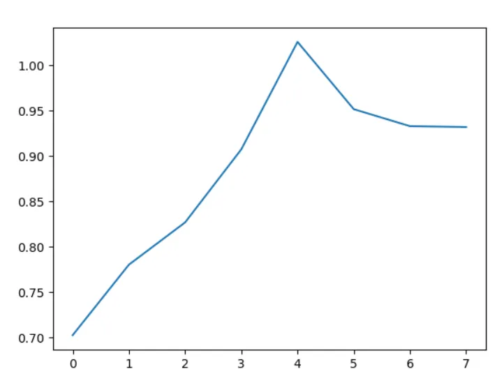
算法结果及评估

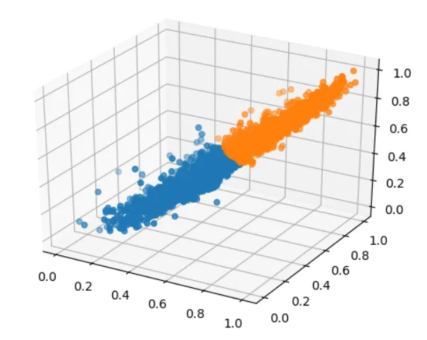
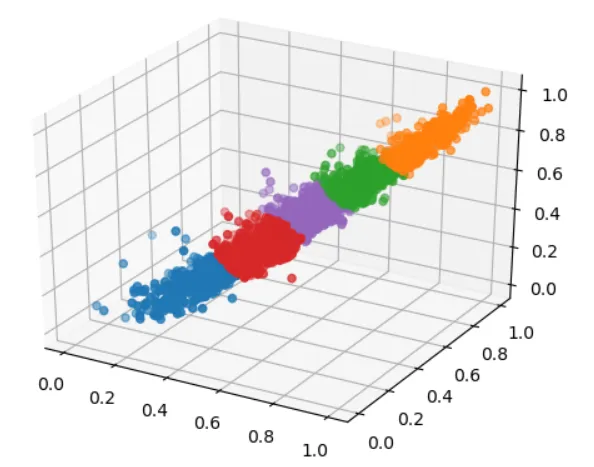
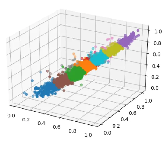
为了更直观的看到分类结果,将分类的点在三维空间中绘制出,用不同的颜色表示不同的类别。

绘图函数如下:

1
2
3
4
5
6
7
8
9
10
11
12
def show_k_means(k_result):
k,k_categories,dire=k_result['k'],k_result['k_categories'],k_result['dire']
for i in range(k):
x,y,z=[],[],[]
for index in k_categories[i]:
x.append(dire[index][0])
y.append(dire[index][1])
z.append(dire[index][2])
fig = plt.gcf()
ax = fig.gca(projection='3d')
ax.scatter(x,y,z)
plt.show()

分类结果如下:

k=2
k=5
k=10

为了更好的评估分类效果,选取DB指数(Davies-Bouldin Index)对分类效果进行评估,DB指数的及算法方法如下:

  • 设一共有\(k\)个簇,每个簇的中心点为\(u_i\),簇中的点用\(x_{ij}\)表示
  • 计算出每个簇的簇内平均距离\(\mu_i\),即簇内所有点到簇中心的平均距离
  • 计算出质心之间的距离\(d(u_i,u_j)\)
  • 计算DBI:

\[ DB=\frac1k\sum_{i=1}^k\mathop{max}\limits_{i\neq j}(\frac{\mu_i+\mu_j}{d(u_i,u_j)}) \]

实现代码如下:

1
2
3
4
5
6
7
8
9
10
11
12
13
14
15
16
17
18
19
20
21
22
23
24
25
def dbi(k_result):
k_center,k_categories,dire,k=k_result['k_center'],k_result['k_categories'],k_result['dire'],k_result['k']
# 簇内平均距离
k_ave_dist=[0 for index in range(k)]
for i in range(k):
temp=0
for item in k_categories[i]:
temp+=distance(k_center[i],dire[item])
k_ave_dist[i]=temp/len(k_categories[i])
# 簇中心之间距离
k_center_dist=[[0 for row in range(k)] for col in range(k)]
for i in range(k):
for j in range(k):
k_center_dist[i][j]=distance(k_center[i],k_center[j])
# 计算dbi
DB=0
for i in range(k):
Max=0
for j in range(k):
if i !=j:
temp=(k_ave_dist[i]+k_ave_dist[j])/k_center_dist[i][j]
if temp>Max:
Max=temp
DB+=Max
return DB/k

计算k=2-10时分类评估结果如下:

k 2 3 4 5 6 7 8 9 10
DBI 0.7028 0.7851 0.8324 0.9075 0.9267 0.9927 0.9242 0.9123 0.8849

k从2-50变化时的分类评估结果如下:

从上述结果可以看出,在k=2或3时的分类效果最好,从使用的数据和k-means算法的特点进行分析,k-means算法采用欧氏距离进行分类,分出的区域为一个个球形。从三维图像上看,采用的数据并没有一个很明显的界限将数据分开,当k=2或3时,每个簇聚集在一个个球中,表现出较好的分类结果。当k继续增长时,由于数据周围孤立点的影响,使分类效果逐渐变差。