Posted onEdited onInStudyViews: Waline: Word count in article: 5.4kReading time ≈5 mins.
This is an automatically translated post by LLM. The original post is in Chinese.
If you find any translation errors, please leave a comment to help me
improve the translation. Thanks!
Overview of BP Neural
Network
The BP neural network is the most basic and widely used neural
network in the field. It consists of three layers of nodes: the input
layer, the hidden layer, and the output layer. The implementation of the
BP neural network is relatively simple, mainly divided into two parts:
forward propagation and backward propagation of errors.
The universal approximation theorem of neural networks states that a
one-dimensional step function can approximate any one-dimensional
continuous function, and a sigmoid function can approximate a step
function. Therefore, a linear combination of one-dimensional sigmoid
functions can approximate any continuous function. This provides a
theoretical basis for the application of neural networks.
The advantage of neural networks lies in the fact that many complex
function mappings that are difficult to solve can be obtained by
combining multiple one-dimensional step functions. The main problem and
difficulty in building a neural network is how to combine these
one-dimensional functions.
Understanding BP Neural
Network
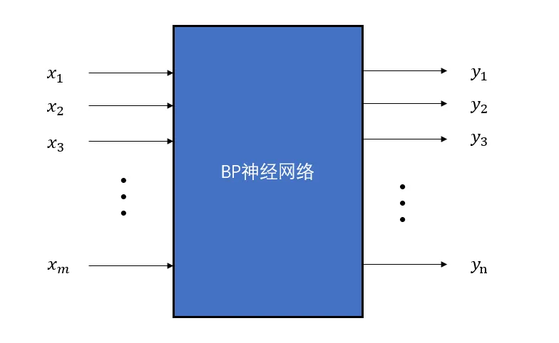
The BP neural network can be seen as a multi-input multi-output
function. If we ignore its internal structure, it can be represented as
a black box model:
Black box model of BP neural
network
In this BP neural network, there are \(m\) inputs and \(n\) outputs. We know that there should be a
hidden layer between the input and output layers. So how many nodes
should be in the hidden layer? Generally, the determination of the
hidden layer is determined by the following empirical formula: \[
h=\sqrt{m+n}+a
\] where \(h\) is the number of
nodes in the hidden layer, \(m\) is the
number of nodes in the input layer, \(n\) is the number of nodes in the output
layer, and \(a\) is an adjustment
constant.
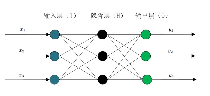
Based on the number of input and output nodes, we can construct a
simple BP neural network model. Its internal structure is as follows
(taking \(m=3\), \(n=3\), and \(h=3\) as an example):
Internal structure of a three-layer
neural network
With such a three-layer neural network, any 3D-to-3D mapping can be
achieved through the combination of one-dimensional functions. So how to
establish this mapping? This problem is actually how to train the BP
neural network. The training process mainly consists of two parts:
forward propagation of results and backward propagation of
residuals.
Forward Propagation
For any node in the BP neural network, its input is the weighted sum
of the outputs of the previous layer nodes. Taking the hidden layer as
an example, let the output of the input layer node be \(x_i\), the input of the hidden layer node
be \(net_j\), the weight connecting
node \(i\) in the input layer to node
\(j\) in the hidden layer be \(w_{ij}\), and the constant term be \(b_j\). Then the input of the hidden layer
node is: \[
net_j=\sum_{i=1}^m w_{ij}x_i+b_j
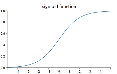
\] In the BP neural network, in order to ensure that the
activation function is differentiable everywhere, the sigmoid function
is used as the activation function. The output of the node is: \[
f(net_j)=\frac1{1+e^{-net_j}}
\]
Advantages of using sigmoid function:
Compared to the step function, it is differentiable everywhere in
its domain.
Let \(y=sigmoid(x)\), then \(y'=y(1-y)\). It can be seen that the
derivative of the sigmoid function can be represented using itself. Once
the value of the sigmoid function is calculated, it is very convenient
to calculate the value of its derivative. This provides convenience for
using gradient descent in backpropagation.
Main disadvantages of the sigmoid function:
Vanishing gradient: Note that when the sigmoid function
approaches 0 or 1, the rate of change becomes flat, which means that the
gradient of the sigmoid tends to 0. Neurons in the network that use the
sigmoid activation function and have outputs close to 0 or 1 are called
saturated neurons. Therefore, the weights of these neurons will not be
updated. In addition, the weights connected to these neurons will also
be updated slowly. This problem is called the vanishing gradient
problem. Therefore, imagine that if a large neural network contains
sigmoid neurons, and many of them are in a saturated state, the network
cannot perform backpropagation.
Not zero-centered: The output of the sigmoid is not
zero-centered.
High computational cost: The exp() function has a higher
computational cost compared to other nonlinear activation
functions.
Sigmoid function
Each neuron performs this independent calculation, so for a set of
inputs, the neural network can perform calculations to obtain the
corresponding outputs. This is the process of forward propagation.
Backward Propagation
At the beginning, all the weights in the system are randomly
determined. Therefore, in order to make the model tend to the desired
result through learning training data, the weights in the nodes need to
be continuously adjusted. The basic algorithm idea of backward
propagation is the gradient descent algorithm in nonlinear programming,
and the goal of the programming is to minimize the loss function. The
general process is as follows:
Set the loss function. Assuming that all the results of the output
layer are \(d_j\), the loss function is
as follows:
\[
E(w,b)=\frac12\sum_{j=0}^{n-1}(d_j-y_j)^2
\]
Modify the \(w\) and \(b\) from the hidden layer to the output
layer through the loss function. For the weight \(w_{ij}\) from the hidden layer node \(i\) to the output layer node \(j\), the modification is as follows (where
\(\eta\) is the learning rate):
This is basically the idea. The process of calculating partial
derivatives is quite complex, so I won't go into detail here. Just
remember the idea of using gradient descent to minimize the loss
function.