Improved multi-robot area coverage using the Bee Algorithm.
This is an automatically translated post by LLM. The original post is in Chinese. If you find any translation errors, please leave a comment to help me improve the translation. Thanks!
GitHub link: https://github.com/KezhiAdore/MultiRobots_CoverMap
Gitee link: https://gitee.com/KezhiAdore/MultiRobots_CoverMap
1. Introduction
1. Background
Robots are increasingly being used in industries, defense, and scientific and technological fields. They can work in complex and dangerous environments that are monotonous and unstructured. The use of robots greatly improves work efficiency, changes people's lifestyles, brings enormous economic and social benefits, and promotes the development of related disciplines and technologies.
Area coverage refers to the process of exploring and accessing the entire area with robots carrying sensors with a certain detection range, such as lasers and sonars, and completing corresponding tasks. Area coverage is a fundamental task of autonomous mobile robots.
2. Problem Definition:
A group of autonomous mobile robots with limited sensing capabilities collaboratively cover a bounded connected area.
Robots can repeatedly cover a certain position in the area, and the goal is to achieve a certain coverage rate of the area.
Robots complete the task in a distributed and non-centralized manner, determining their actions based on the locally detected information without relying on external control.
The coverage speed should be as fast as possible.
3. Complexity Analysis of the Problem
Compared to general intelligent optimization problems, the swarm robot area coverage problem is more complex in the following aspects:
Dynamics: The problem introduces the time dimension, and the solution obtained is a sequence of robot paths (point sequences), resulting in an extremely large solution space.
Distributed: The execution center of the algorithm is on a single robot, without external host for unified control. The computational and sensing capabilities of a single robot are limited, and the computing power and information used for decision-making are limited.
Large-scale: In order to ensure the accuracy of map representation, the number of grid cells in the grid map must be large. At the same time, the actual environment map is complex and variable, and the area is large, with a large number of robots.
2. Preliminary Model Construction
1. Modeling the Environment
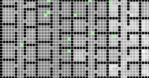
Gridify the map to form a grid map as the environment for robot movement and obstacle placement.
The grid map divides the environment into rectangular grid cells, with each grid cell serving as the smallest unit for robot movement and coverage. Each grid cell has certain attributes, such as the concentration of pheromones, whether it has been covered, and whether it is empty or an obstacle.
There are obstacles distributed in the map, and the robots cannot pass through the obstacle grid cells, but they can be detected by the robots.
2. Modeling the Robots
2.1 Modeling the Robots as Particles
Ignore the physical shape of the robots and treat them as collision-free particles without volume. The robots can only be in one grid cell of the grid map, and multiple robots can exist in the same grid cell.
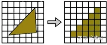
2.2 Modeling the Detection Range of Robots
Due to the limitation of the distributed robot's power supply, its detection range is also limited. To simplify the calculation on the grid map, the detection range of the robot's pheromones is defined as four units in the up, down, left, and right directions.
2.3 Functions of Robots
Robots can perform the following operations: move to one of the four directions of up, down, left, and right or stay still, perceive the grid cells in the up, down, left, right, and current positions, and modify the concentration of pheromones in the grid cell they are in.
We focus more on the influence of pheromones on robot behavior rather than studying the specific pheromones used for communication in physical terms. Therefore, the concentration of pheromones at each position is abstracted as a number, and the robot can modify the concentration of pheromones when it reaches that position.
3. Modeling Time
Discretize time into units called "rounds". In each round, each robot performs the following actions:
Step 1: Achieve coverage of the current grid cell.
Step 2: Modify the concentration of pheromones in the current grid cell.
Step 3: Perform a movement or choose to stay still.
All robots perform these three actions synchronously in each round.
4. Modeling the Solution to the Problem
4.1 Representation of the Solution
For a grid cell, it can be represented by a pair of coordinates \((x, y)\). If the coverage process lasts for t rounds and involves n robots, the solution can be represented by a sequence of grid cells with a length of t for each robot, representing the movement trajectory of each robot. The valid solution should not include obstacle grid cells. The set of all grid cells forms the covered grid cells.
4.2 Evaluation of the Solution
We define coverage rate as the ratio of covered grid cells to all grid cells. The target coverage rate is denoted as α. When the current coverage rate exceeds α or the time exceeds the upper limit, the coverage process stops. The quality of the solution is measured by the coverage time t. For maps of the same size and the same number of robots, the shorter the time to achieve the given coverage rate, the better the solution. Multiple experiments are conducted, and the shorter the average time to achieve the given coverage rate, the better the algorithm performance, and the smaller the standard deviation of the average time, the better the algorithm performance.
3. Algorithm Design and Improvement
1. Common Description of the Map and Robots
For this problem, different coverage algorithms have different rules for robot operation. However, the establishment and description of the map are the same and can be reused in different algorithms. The description of the map is as follows: - The map size is M*N, and the total number of robots is n, denoted as r1, r2, ..., ri, ..., rn. - The concentration of pheromones at a point (i, j) on the map is denoted as sij, and the initial concentration of pheromones at each point is 1.
2. Basic Bee Algorithm
The rules for robot operation are as follows:
- The response threshold of each robot is θ.
- For a robot ri at position (xi, yi), first update the concentration of pheromones at its current position:
\[ s_{xiyi} = s_{xiyi} \times \alpha (\alpha \in (0, 1)) \]
- Detect the concentration of pheromones in the surrounding cells: up: s1, down: s2, left: s3, right: s4.
- The probability of robot choosing direction k is:
\[ \frac{s_k^2}{\theta^2 + \sum_{k=1}^{4} s_k^2} \]
- The probability of robot staying still is:
\[ \frac{\theta_i^2}{\theta^2 + \sum_{k=1}^{4} s_k^2} \]
- Use roulette wheel selection to choose the next movement direction or stay still.
The above algorithm is the most basic bee algorithm in the literature, with two parameters θ and α that affect the robot's movement. Through simulation experiments, the influence of these two parameters on map coverage is explored. All simulation maps in this experiment are of size 100*100, with 50 robots randomly distributed on the map.
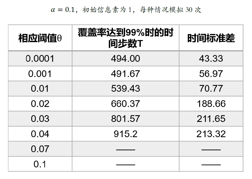
From the above experimental results, it can be seen that as θ increases, the coverage time and time variance increase rapidly. From the perspective of the algorithm, when θ is larger, the robot is more likely to stay still after exploring the surrounding area.
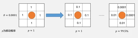
When θ is very small, even if the surrounding cells have been visited multiple times, the robot still has a high probability of moving instead of staying still.
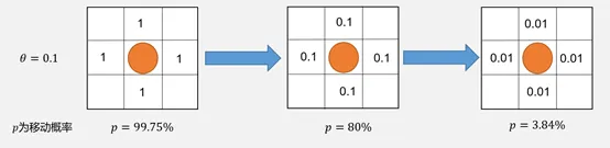
When θ is not much different from the initial concentration of pheromones, such as in the above figure where θ is 1/10 of the initial concentration, in this case, if all four surrounding cells have been visited more than twice, the probability of the robot moving is greatly reduced. This leads to a sharp increase in the average coverage time and variance. Considering the above experimental results and the actual situation, since the effect of the robot staying still when θ is very small is negligible, and when θ is large, it will seriously affect the map coverage speed, in practical applications, we hope that the swarm robots can complete the coverage as quickly as possible rather than saving energy. Therefore, we choose to remove the rule of robots staying still, that is, θ=0. After the above modification, further experiments are conducted to explore the influence of α on the coverage time of swarm robots.
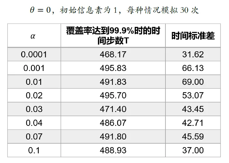
From the above experimental data, it can be seen that with the change of α, the coverage time and coverage time variance do not change much, and there is a trend of increasing and then decreasing. This is because when α is small, the concentration of pheromones in the explored area changes rapidly, effectively preventing repeated exploration. When α is large, there is a certain tolerance for returning to previously explored areas, allowing robots to return to the original area to cover the missed area. Both have their advantages and disadvantages, but overall, the value of α has little impact on coverage efficiency.
3. Bee Algorithm with Adaptive Pheromone Release
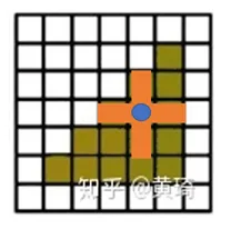
Through the analysis of the above bee algorithm, we found that the following two situations have the same change in the concentration of pheromones in the central area under the bee algorithm.
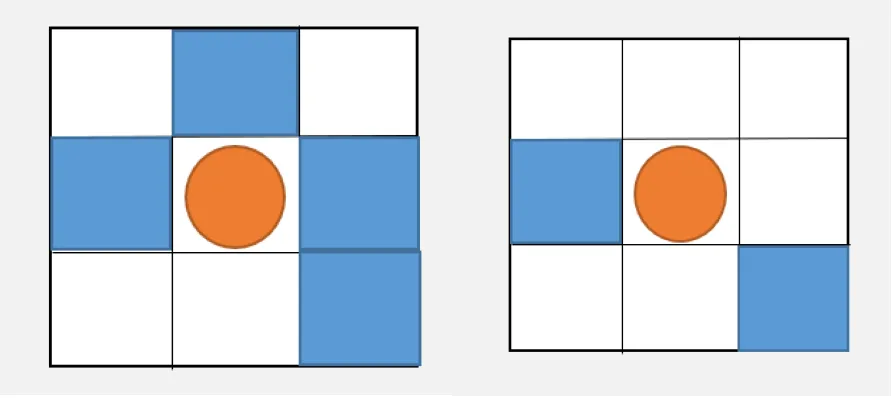
However, in reality, for the scenario on the right, in order to explore the blank cells around the central node, we hope that some robots can return to the central node. For the scenario on the left, since its surroundings have been mostly explored, it is not meaningful for robots to return to the central node, and we hope that robots will try to avoid returning to that area. Therefore, we propose an adaptive pheromone release method, where the modification of pheromones is small when there are many unexplored cells around, and the modification of pheromones is large when there are few unexplored cells. At the same time, we hope that this change is nonlinear. The new pheromone release method is as follows:
- The basic update of pheromones is still: \[ s = s \times \alpha \]
- Let m be the number of empty cells around a certain cell, then the weight exponent to be added is: \[ k = 1 + \frac{4-m}{4} \]
- Then the way robots update pheromones in a certain cell becomes: \[ s = s \times \alpha^k \]
4. Bee Algorithm with Memory Backtracking
In obstacle map coverage tests, we found the following phenomenon: robots are trapped in a small enclosed area with a small entrance and cannot get out. This leads to robots being trapped and unable to work properly.
To avoid this situation, we consider the backtracking feature of depth-first search (DFS) and perform backtracking when there is no way out. The algorithm flow combining memory backtracking with the bee algorithm is as follows:
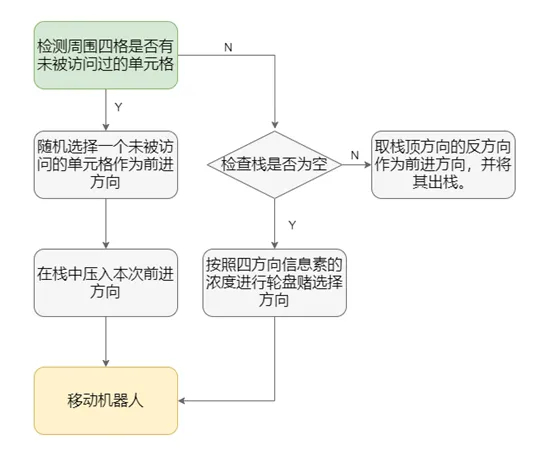
Using this algorithm, even if the robot enters a local obstacle area, it can use the memory path to backtrack and walk out of the local environment, which has good reliability and robustness.
4. Performance Testing and Improvement Direction
1. Testing on Open Maps
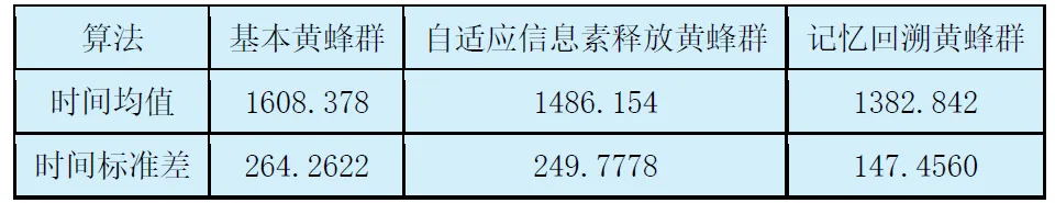
Open maps are the simplest and most convenient maps to test, and the test results on these maps can well reflect the time and time stability of the algorithms mentioned above. At the same time, in this experiment, the number of tests is increased, with each map and each algorithm tested 500 times to avoid randomness. The test results on open maps are as follows:
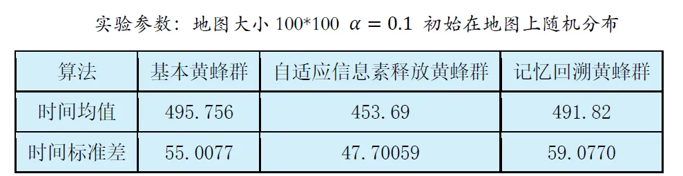
From the above experimental results, it can be seen that the adaptive pheromone release bee algorithm has the shortest exploration time and the best time stability. The other two algorithms have similar coverage times, and the time stability of the memory backtracking bee algorithm is slightly worse.
2. Testing on Maps with Simple Obstacles
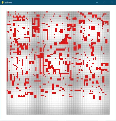
The test results on the above map are as follows:
The test results are significantly different from those on open maps. The memory backtracking bee algorithm performs the best in terms of the two evaluation metrics, followed by the adaptive pheromone release bee algorithm. The basic bee algorithm takes longer and has worse time stability.
3. Testing on Real Terrain
3.1 Hot Spring Bathroom
The map of the hot spring bathroom is as follows:
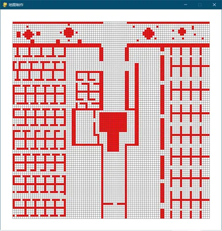
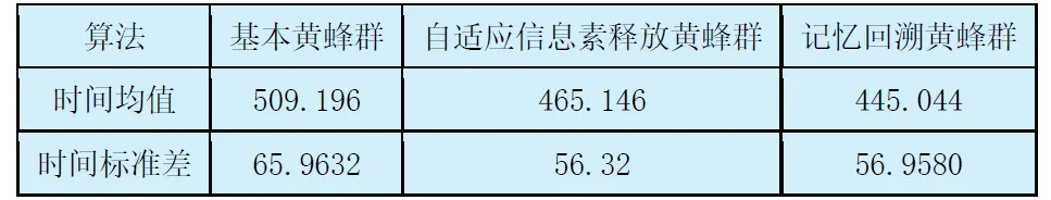
The most notable feature of this map is the presence of many small rooms with small entrances, making it easy for robots to get trapped and unable to get out. The results of the three algorithms on this map are as follows:
Due to the influence of the terrain and in order to test the actual environment, all robots start from the top left corner of the map instead of being randomly distributed initially, resulting in a significant increase in the time required for the three algorithms to cover the map.
From the three sets of results, the memory backtracking bee algorithm has the highest efficiency, followed by the adaptive pheromone release bee algorithm, and the basic bee algorithm takes the longest time and has the worst time stability.
3.2 Zhongying College
The terrain of Zhongying College is as follows:
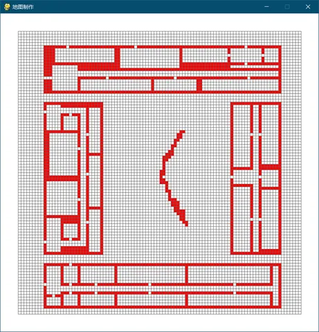
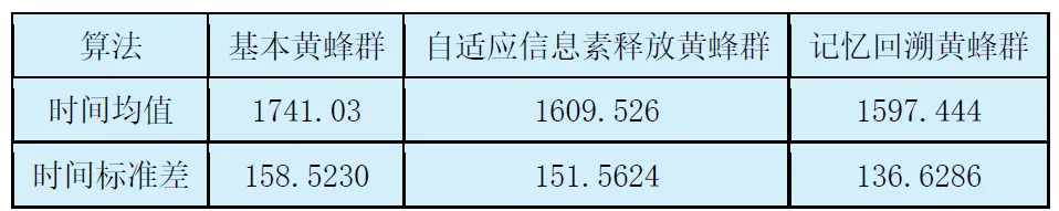
The test results are as follows:
In this map, the memory backtracking bee algorithm is obviously superior to the other two intelligent algorithms, and the adaptive pheromone release algorithm is also more efficient than the basic bee algorithm. The basic bee algorithm takes longer and has worse time stability.
4. Experimental Conclusion
The bee algorithm with heuristic pheromone release is more time-efficient than the basic bee algorithm in all cases.
The bee algorithm with memory backtracking performs best in maps with many obstacles, followed by the adaptive pheromone release bee algorithm. The basic bee algorithm takes longer and has worse time stability.
5. Other Improvement Ideas
Bee Algorithm with Limited-Length Memory for Depth-First Search
In practical situations, unlimited memory for the DFS algorithm is difficult to achieve due to movement errors and memory limitations. Therefore, a length limit can be added to the algorithm.
- Queue length limit: Use a deque instead of a stack, and pop the last element when the queue length exceeds the limit.
- Stack length limit: Force backtracking when the stack length exceeds the limit.