Digital Image Processing (6) Frequency Domain Filters.
This is an automatically translated post by LLM. The original post is in Chinese. If you find any translation errors, please leave a comment to help me improve the translation. Thanks!
Introduction to Frequency Domain Filters
Frequency domain filters are different from spatial domain filters. Spatial domain filters perform convolution operations between spatial convolution kernels and spatial images, while frequency domain filters perform multiplication operations between the frequency domain image obtained by discrete Fourier transform (DFT) and the filter in the frequency domain, and then perform inverse Fourier transform (IDFT) to obtain the filtered image.
The basic steps of using frequency domain filters to filter images are as follows:
- Perform DFT on the image to obtain the frequency domain image of the original image.
- Multiply the frequency domain image by the frequency domain filter to obtain a new frequency domain image.
- Perform IDFT on the new frequency domain image to obtain a new image in the spatial domain.
There are several things to note:
- When performing DFT, the original image is extended periodically in the spatial domain. If the original image is directly used for DFT, the DFT result will be calculated based on the original image surrounding the four sides. Therefore, to eliminate the edge effects of the filtered result, the image can be transformed to four times the size of the original image, and the original image is placed in the upper left corner of the four times image, with zero padding in other places.
- For convenience of calculation, the origin (0,0) of the frequency domain image is generally placed at the center of the image. However, the (0,0) point of the frequency domain image obtained by directly performing DFT on the image is located at the four corners of the image. To move the (0,0) point of the frequency domain image, each pixel of the spatial domain image should be multiplied by \((-1)^{i+j}\) before DFT (\(i\) and \(j\) are the horizontal and vertical coordinates with the upper left corner of the image as the origin and the right and down directions as positive directions). Of course, this operation is performed during the transformation, and it should be restored after the inverse transformation.
The function for zero-padding the image, performing DFT, and transforming the center of the frequency domain image is as follows:
1 | def fft(img): # Perform 2D fast Fourier transform on the image |
The function for performing the corresponding inverse transformation on the frequency domain image is as follows:
1 | def ifft(f_img): # Perform 2D inverse Fourier transform |
Frequency Domain Low Pass Filters
As the name suggests, a low pass filter allows low frequencies to pass through and blocks high frequencies. If the origin of the frequency domain is placed at the center of the image, the ideal low pass filter is represented as:

However, this filter is discontinuous at the boundaries, making it impossible to implement with physical devices. Even if it is simulated on a computer, it will still have some impact on the image. Therefore, this ideal filter is generally not used.
Gaussian Low Pass Filter
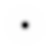
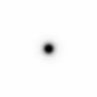
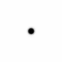
The Gaussian low pass filter (GLPF) is one of the most commonly used low pass filters. It is generated by a two-dimensional Gaussian function, and its mathematical expression is: \[ H(u,v)=e^{-D^2(u,v)/2D_0 ^2} \] where \(D(u,v)\) is the distance from a point in the image to the center of the image, and \(D_0\) is the cutoff frequency. When \(D(u,v)=D_0\), the GLPF drops to 0.607, which is its maximum value. The filter is represented by the following images (with cutoff frequencies of 10, 30, and 60):
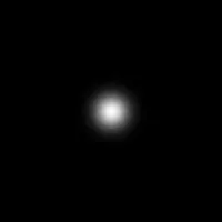
|
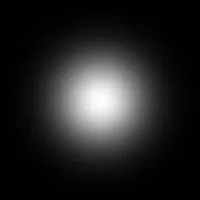
|

|
The function for generating the Gaussian filter is as follows:
1 | def gauss_filter(shape, D0): # Generate a Gaussian low pass filter with a cutoff frequency of D0 |
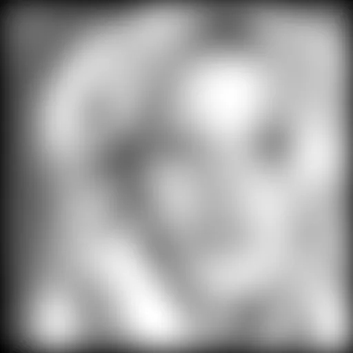
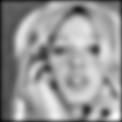
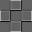
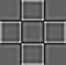
The filtered image using the Gaussian low pass filter is as follows (original image, Gaussian filters with radii of 10 and 20):
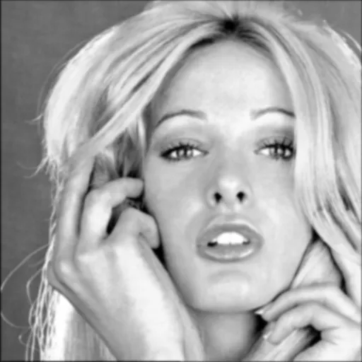 |
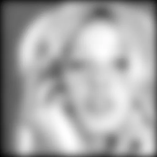 |
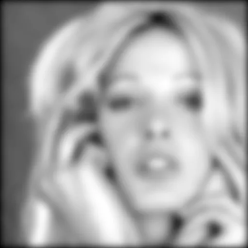 |
The function for filtering the image using the Gaussian low pass filter is as follows:
1 | def gaussian(img, D0): # Filter the image using a Gaussian low pass filter of order n and cutoff frequency D0 |
Butterworth Low Pass Filter
The transfer function of an \(n\)-th order Butterworth low pass filter (BLPF) with a cutoff frequency at a distance of \(D_0\) from the origin is defined as: \[ H(u,v)=\frac 1{1+[D(u,v)/D_0]^{2n}} \] The Butterworth filter is represented by the following images (with \(n=1,2,5\)):
 |
 |
 |
The function for generating the Butterworth filter is as follows:
1 | def butter_filter(shape, n, D0): # Generate an n-th order Butterworth low pass filter with a radius of D0 |
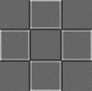
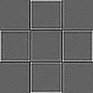
The filtered image using the Butterworth low pass filter is as follows (original image, Butterworth filters with orders of 3 and radii of 10 and 20):
|
|
 |
 |
The function for filtering the image using the Butterworth low pass filter is as follows:
1 | def butterwroth(img, n, D0): # Filter the image using an n-th order Butterworth filter with a cutoff frequency D0 |
Frequency Domain High Pass Filters
In contrast to low pass filters, high pass filters block low frequencies and allow high frequencies to pass through. The ideal high pass filter is represented as:

Gaussian High Pass Filter
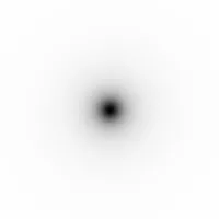
The Gaussian high pass filter (GHPF) with a cutoff frequency of \(D_0\) is defined as: \[ H(u,v)=1-e^{-D^2(u,v)/2D_0 ^2} \] The filter is represented by the following images (with image size of 200*200 and cutoff frequencies of 5, 10, and 30):
|
|

|
The function for generating the Gaussian high pass filter is as follows:
1 | def gauss_filter(shape, D0): # Generate an n-th order Gaussian high pass filter with a cutoff frequency of D0 |
The filtered image using the Gaussian high pass filter is as follows (original image, Gaussian filters with radii of 10 and 30):

|
|
|
Butterworth High Pass Filter
The \(n\)-th order Butterworth high pass filter (BHPF) with a cutoff frequency at a distance of \(D_0\) from the origin is defined as: \[ H(u,v)=\frac 1{1+[D_0/D(u,v)]^{2n}} \] The filter is represented by the following images (with image size of 200*200, cutoff frequency of 10, and orders of 1, 2, and 4):
|
|
|
The function for generating the Butterworth high pass filter is as follows:
1 | def butter_filter(shape, n, D0): # Generate an n-th order Butterworth high pass filter with a radius of D0 |
The filtered image using the Butterworth high pass filter is as follows (original image, Butterworth filters with orders of 3 and radii of 10 and 30):
|
|
|
|
References
[1] Rafael C. Gonzalez and Richard E. Woods, "Digital Image Processing", 3rd Edition, Beijing: Publishing House of Electronics Industry, 2017.5
[2] lcxxcl_1234, "numpy中的fft和scipy中的fft,fftshift以及fftfreq" [Online]. CSDN: 2018-07-02 [2020-04-05]. Available: https://blog.csdn.net/lcxxcl_1234/article/details/80889783
[3] Ke Ming Fang, "The Difference Between Power Spectrum and Frequency Spectrum" [Online]. CSDN: 2017-08-10 [2020-04-06]. Available: https://blog.csdn.net/godloveyuxu/article/details/77030793