线性滤波与非线性滤波实验
本文围绕自由落体运动的估计,进行了线性滤波和非线性滤波的实验。下面这张图是源自西安交通大学蔡远利教授的《随即滤波与控制》课程。 该课程主要围绕估计,平滑与预测三方面讲解各类滤波方法。
问题描述
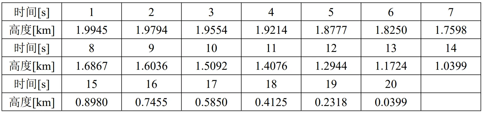
已知一物体作自由落体运动,对其高度进行了20次测量,测量值如下表:
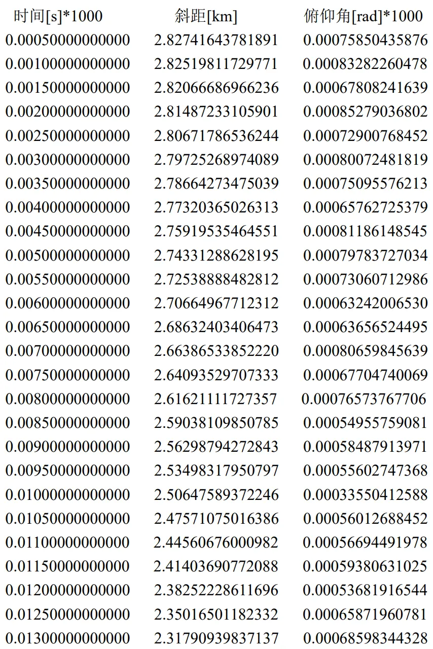
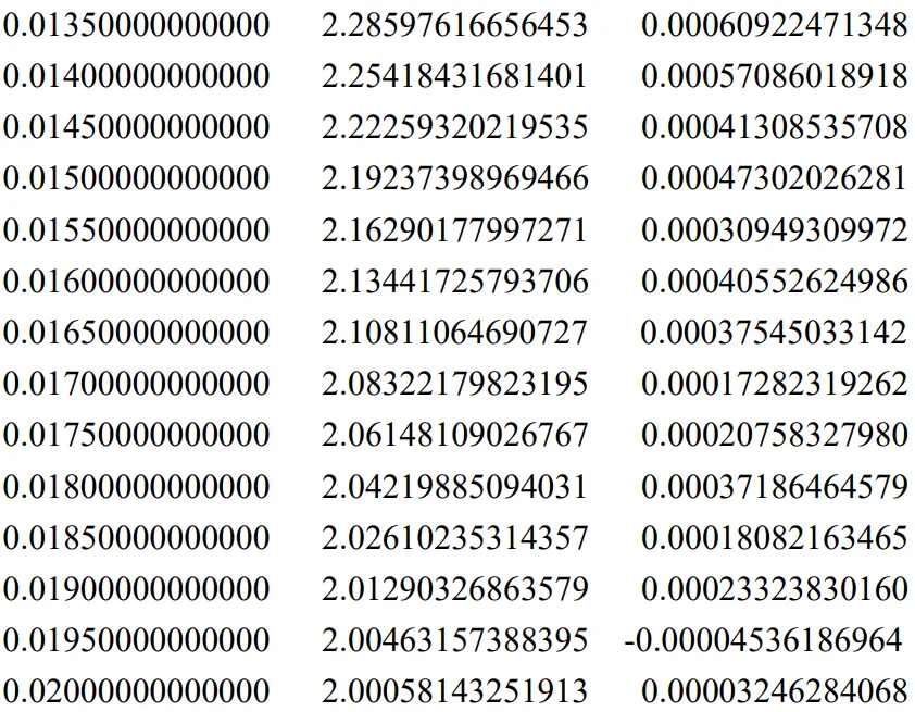
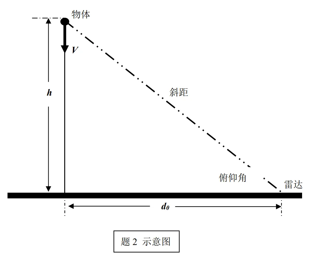
同样考虑自由落体运动的物体,用雷达(和物体在同一水平面)进行测量,如图所示,如果雷达测距和测角的量测噪声为高斯白噪声序列,均值为0,方差阵 \(R=\begin{bmatrix}0.04 &0\\0&0.01\end{bmatrix}\),试根据以下测量数据确定物体的高度和下落速度随时间变化的估计值:
该下落运动和雷达检测信息如下图所示:
模型介绍
1. 线性估计问题
设在自由落体运动时,物体高度为 \(h\),速度为 \(v\) (向下为正),设 \(x_1=h,x_2=v\),则系统的状态方程为:
\[ \begin{bmatrix} \dot x_1\\\dot x_2 \end{bmatrix}= \begin{bmatrix} 0&-1\\ 0&0\\ \end{bmatrix} \begin{bmatrix} x_1\\x_2 \end{bmatrix}+ \begin{bmatrix} 0\\1 \end{bmatrix}g\ \ (g=9.80m/s^2) \]
由上述状态方程可以解出系统的状态转移函数为:
\[ x(t)=\begin{bmatrix} 1&-t\\ 0&1 \end{bmatrix}x(0) +\begin{bmatrix} -t\\1 \end{bmatrix}u(t) \]
当步长为 1s 时系统的状态转移函数为:
\[ \Phi_{k+1,k}=\begin{bmatrix} 1&-1\\ 0&1 \end{bmatrix} \ \Psi_{k+1,k}=\begin{bmatrix} -1\\ 1 \end{bmatrix} \]
由此可得,系统的一步预测为:
\[ x_{k+1,k}=\Phi_{k+1,k}x_{k|k}+\Psi_{k+1,k}u_k \]
由于观测是对物体高度的直接测量,并且假设量测误差为均值为0,方差为1的白噪声,则量测方程为: \[ y_k=H_kx_k+v_k \]
其中: \[ H_k\equiv \begin{bmatrix} 1\\0 \end{bmatrix}, \ v_k \sim N(0,1), \ R=1 \]
本题给出的数据中,量测高度单位为\(km\),加速度为\(9.8m/s\),为便于计算,统一距离单位为\(km\),时间单位统一为\(s\),即重力加速度\(g=0.0098km/s\)。由于滤波初值未给定,根据量测数据估算初始高度为\(2km\),初始速度为0,即\(x_{0|0}=\begin{bmatrix}2&0\end{bmatrix}\)。由于这样确定的初始估计值比较粗糙,因此方差较大,设定系统初始方差阵为\(P_{0|0}=\begin{bmatrix}10&0\\0&10\end{bmatrix}\)。
建立卡尔曼滤波: \[ x_{k+1,k}=\Phi_{k+1,k}x_{k|k}+\Psi_{k+1,k}u_k\\ P_{k+1|k}=\Phi_{k+1,k}P_{k|k}\Phi^\top_{k+1,k}\\ P_{k+1|k+1}=[P_{k+1|k}^{-1}+H_{k+1}^{\top} R_{k+1}^{-1}H_{k+1}]^{-1}\\ K_{k+1}=P_{k+1|k+1}H_{k+1}^\top R_{k+1}^{-1}\\ \hat x_{k+1|k+1}=\hat x_{k+1|k}+K_{k+1}(y_{k+1}-H_{k+1}\hat x_{k+1|k}) \] 对物体自由落体下降高度和速度进行计算,计算结果见后文实验结果部分。
2. 非线性估计问题
在第2个问题中,量测与估计值为非线性关系,考虑采用非线性卡尔曼滤波算法对其进行估计,本报告中采用扩展式卡尔曼滤波算法(EKF)。
设测量的斜距为\(l(km)\),俯仰角为\(\theta(rad)\),物体高度为\(h(km)\),下降速度为\(v(km/s)\)(向下为正),物体在地面上的竖直投影到雷达的距离为\(d_0\)。
为便于后续线性化计算,选取系统状态量为: \[ x_1=h,\ x_2=v,\ x_3=d_0 \] 则系统的状态方程为: \[ \dot x= \begin{bmatrix} 0&-1&0\\ 0&0&0\\ 0&0&0 \end{bmatrix}x+ \begin{bmatrix} 0\\ 1\\ 0 \end{bmatrix}g,\ 其中\ g=0.0098\ km/s \] 求解得出当时间间隔为\(0.5s\)时,系统的离散状态转移函数为: \[ \Phi_{k+1,k}=\begin{bmatrix} 1&-0.5&0\\ 0&1&0\\ 0&0&1 \end{bmatrix},\ \Psi_{k+1,k}=\begin{bmatrix} -0.125\\ 0.5\\ 0 \end{bmatrix} \] 系统观测为雷达测量出的斜距和俯仰角,则: \[ y_1=l=\sqrt{h^2+d_0^2}=\sqrt{x_1^2+x_3^2}\\ y_2=\theta=\arctan(\frac{h}{d_0})=\arctan(\frac{x_1}{x_3}) \] 观测量对状态量求导可得: \[ \frac{\partial y_1}{\partial x_1}=\frac{x_1}{\sqrt{x_1^2+x_3^2}}\\ \frac{\partial y_1}{\partial x_2}=0\\ \frac{\partial y_1}{\partial x_3}=\frac{x_3}{\sqrt{x_1^2+x_3^2}}\\ \frac{\partial y_2}{\partial x_1}=\frac{x_3}{x_1^2+x_3^2}\\ \frac{\partial y_2}{\partial x_2}=0\\ \frac{\partial y_2}{\partial x_3}=-\frac{x_1}{x_1^2+x_3^2}\\ \] 因此,系统的局部线性化系数为: \[ H=\begin{bmatrix} \frac{x_1}{\sqrt{x_1^2+x_3^2}}&0&\frac{x_3}{\sqrt{x_1^2+x_3^2}}\\ \frac{x_3}{x_1^2+x_3^2}&0&-\frac{x_1}{x_1^2+x_3^2} \end{bmatrix} \] 扩展卡尔曼滤波(EKF)的计算过程如下: \[ x_{k+1,k}=\Phi_{k+1,k}x_{k|k}+\Psi_{k+1,k}u_k\\ P_{k+1|k}=\Phi_{k+1,k}P_{k|k}\Phi^\top_{k+1,k}\\ P_{k+1|k+1}=[P_{k+1|k}^{-1}+H_{k+1}^{\top} R_{k+1}^{-1}H_{k+1}]^{-1}\\ K_{k+1}=P_{k+1|k+1}H_{k+1}^\top R_{k+1}^{-1}\\ \hat x_{k+1|k+1}=\hat x_{k+1|k}+K_{k+1}(y_{k+1}-H_{k+1}\hat x_{k+1|k}) \] 其中,与卡尔曼滤波不同的地方在于\(H\)系数矩阵是通过在观测点进行局部线性化得到的。通过上述步骤即可对非线性观测进行滤波估计。
实验结果
1. 线性滤波问题
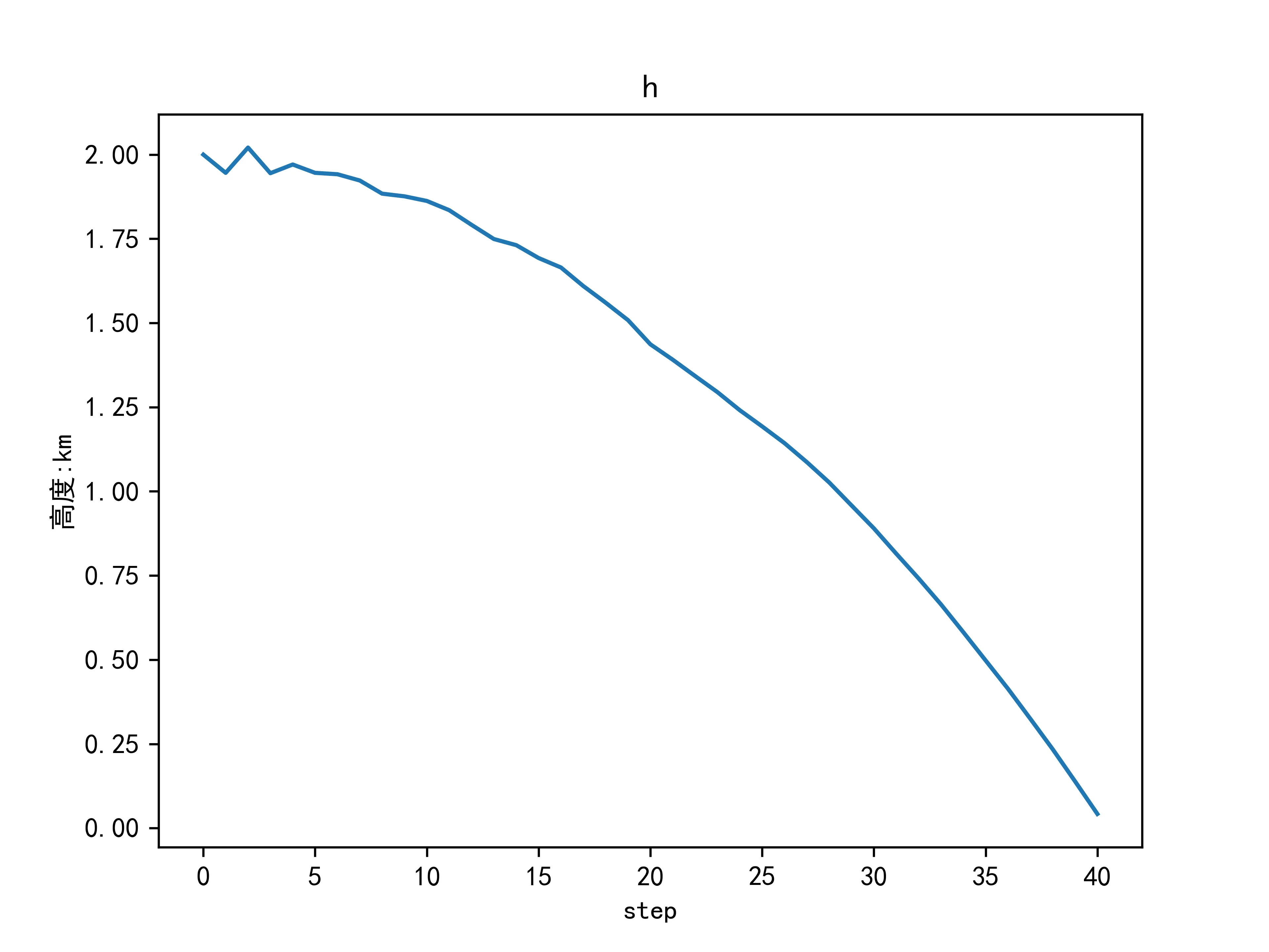
根据题中给出的高度观测数据进行线性卡尔曼滤波,计算得到的结果如下:
高度估计数据为:
| 时间 | 1 | 2 | 3 | 4 | 5 | 6 | 7 |
|---|---|---|---|---|---|---|---|
| 高度 | 1.9943 | 1.9791 | 1.9550 | 1.9211 | 1.8774 | 1.8244 | 1.7605 |
| 时间 | 8 | 9 | 10 | 11 | 12 | 13 | 14 |
|---|---|---|---|---|---|---|---|
| 高度 | 1.6870 | 1.6038 | 1.5103 | 1.4075 | 1.2947 | 1.1723 | 1.0400 |
| 时间 | 15 | 16 | 17 | 18 | 19 | 20 | |
|---|---|---|---|---|---|---|---|
| 高度 | 0.8980 | 0.7460 | 0.5845 | 0.4129 | 0.2317 | 0.0405 |
绘制出高度变化图如下:

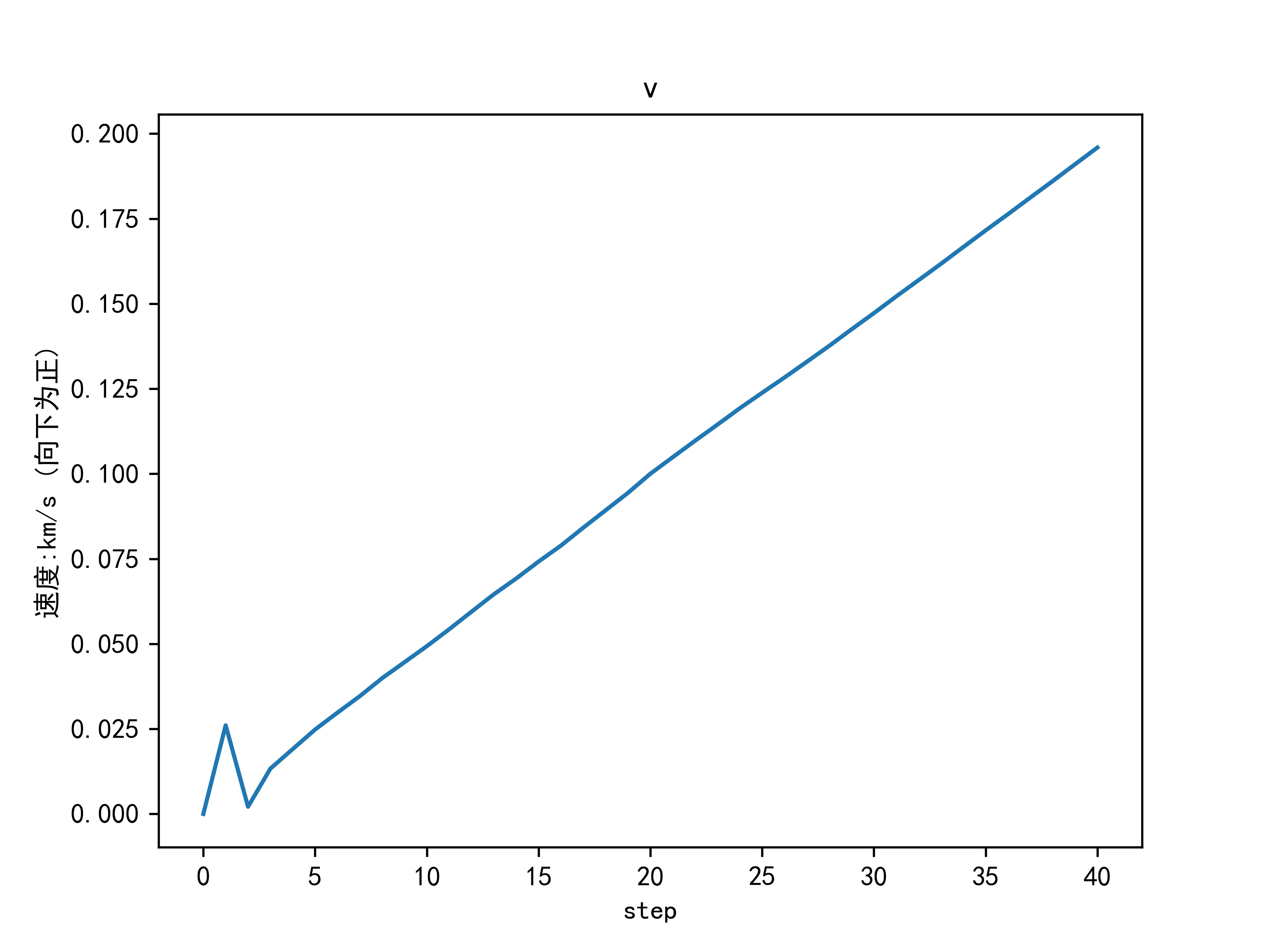
下落速度(向下为正)滤波数据如下表所示:
| 时间 | 1 | 2 | 3 | 4 | 5 | 6 | 7 |
|---|---|---|---|---|---|---|---|
| 下落速度 | 0.0078 | 0.0157 | 0.0247 | 0.0343 | 0.0439 | 0.0536 | 0.0635 |
| 时间 | 8 | 9 | 10 | 11 | 12 | 13 | 14 |
|---|---|---|---|---|---|---|---|
| 下落速度 | 0.0733 | 0.0831 | 0.0930 | 0.1028 | 0.1126 | 0.1224 | 0.1322 |
| 时间 | 15 | 16 | 17 | 18 | 19 | 20 | |
|---|---|---|---|---|---|---|---|
| 下落速度 | 0.1420 | 0.1519 | 0.1616 | 0.1714 | 0.1812 | 0.1911 |
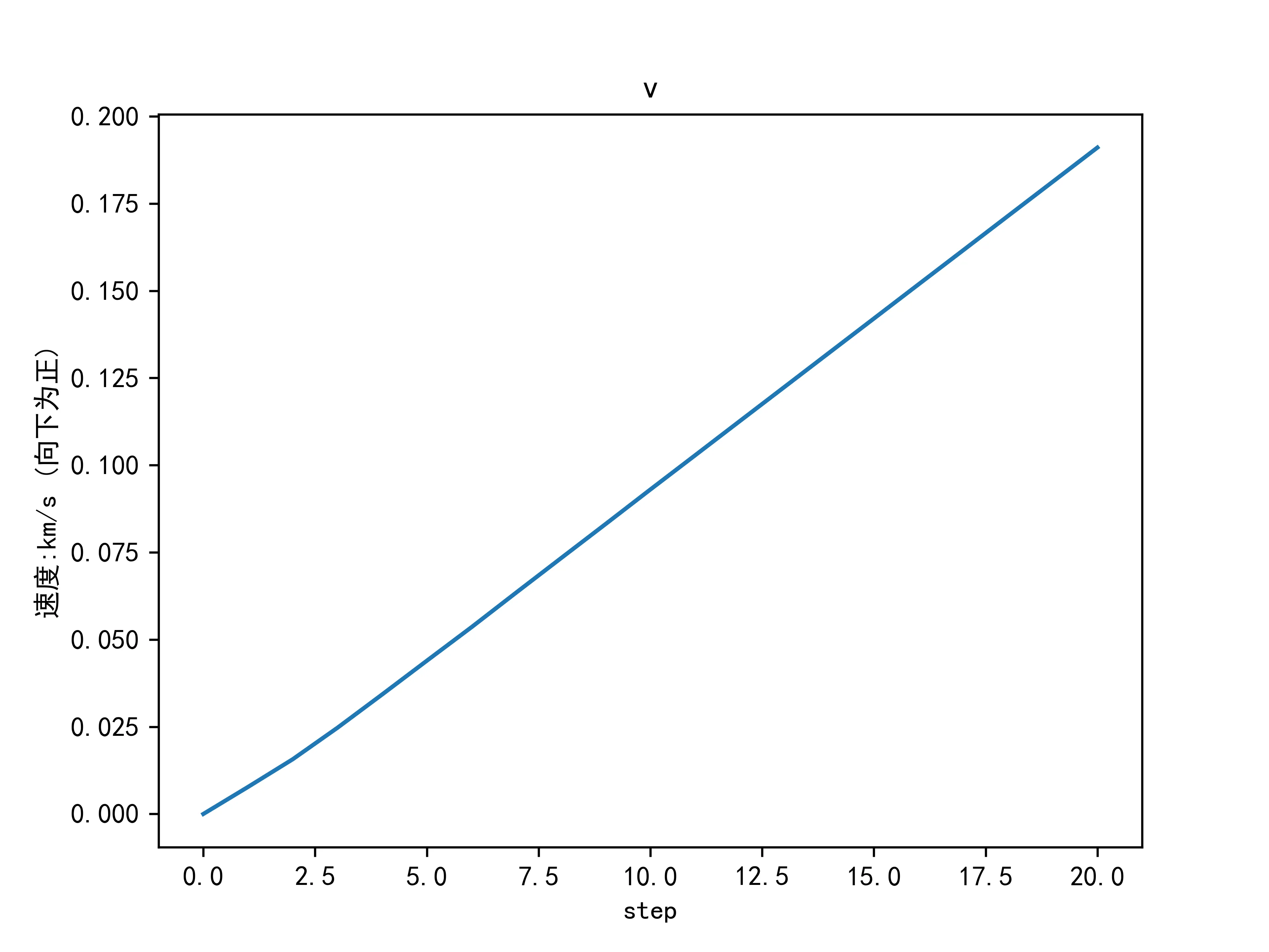
绘制出速度变化图如下:
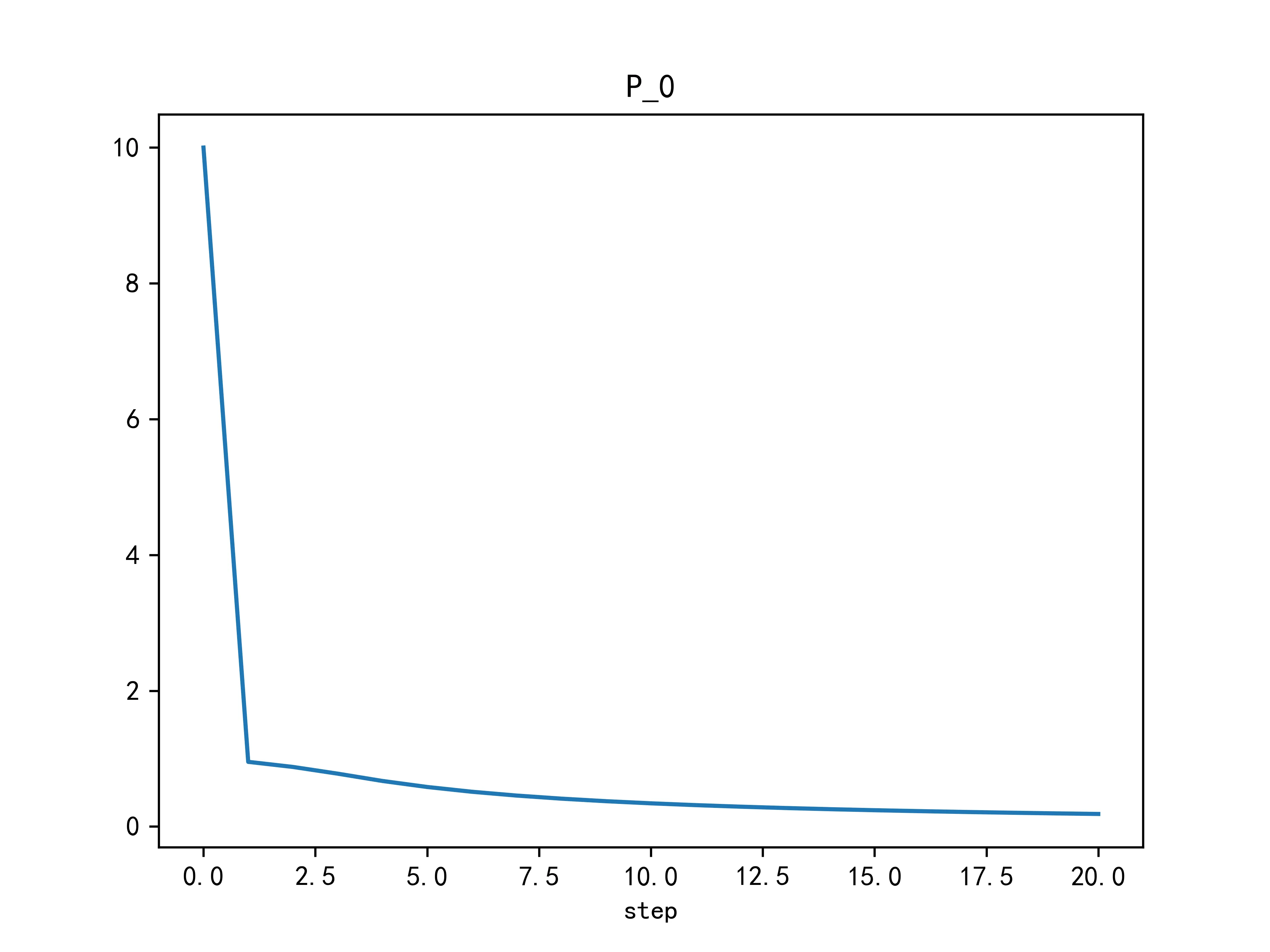
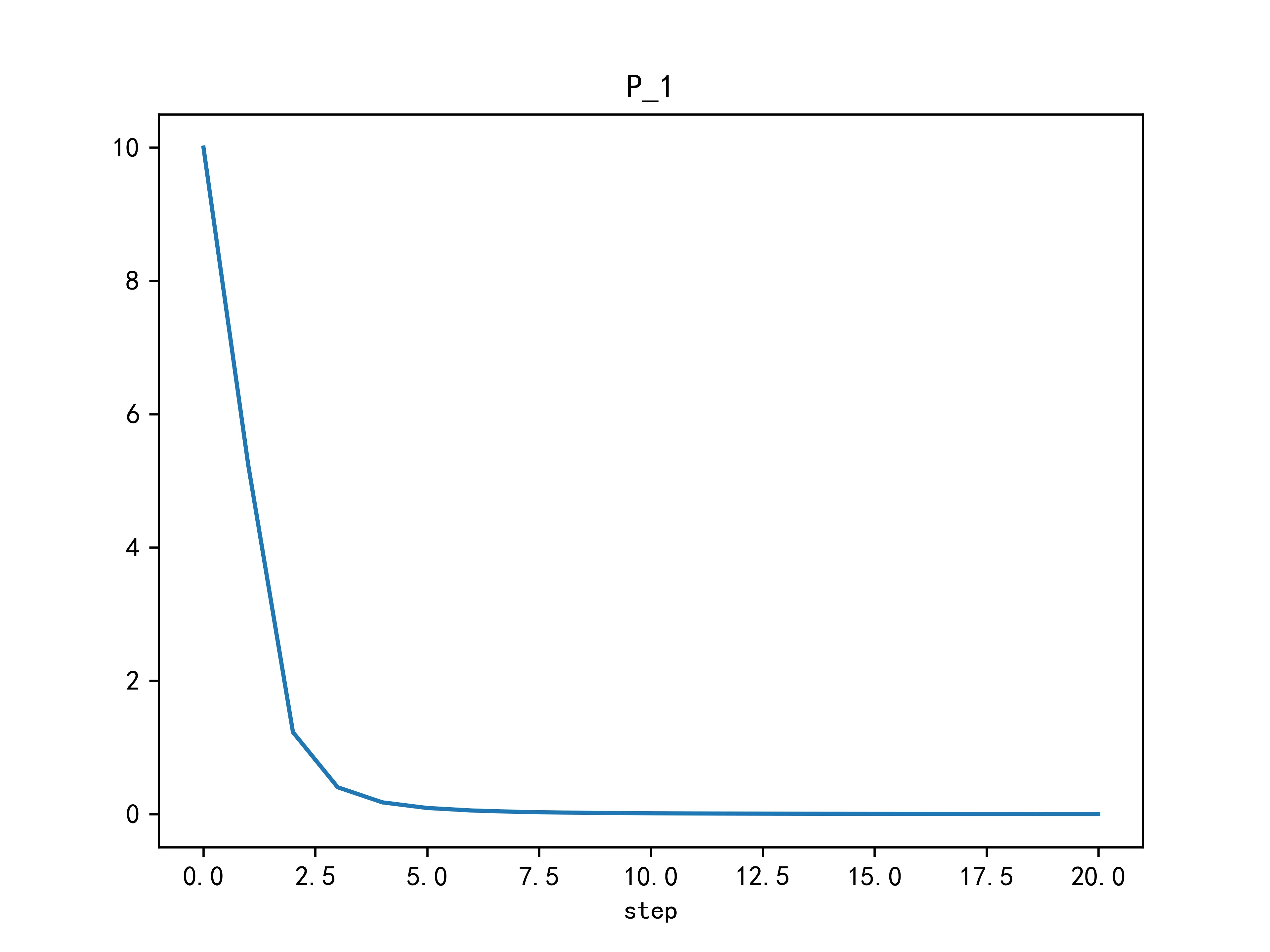
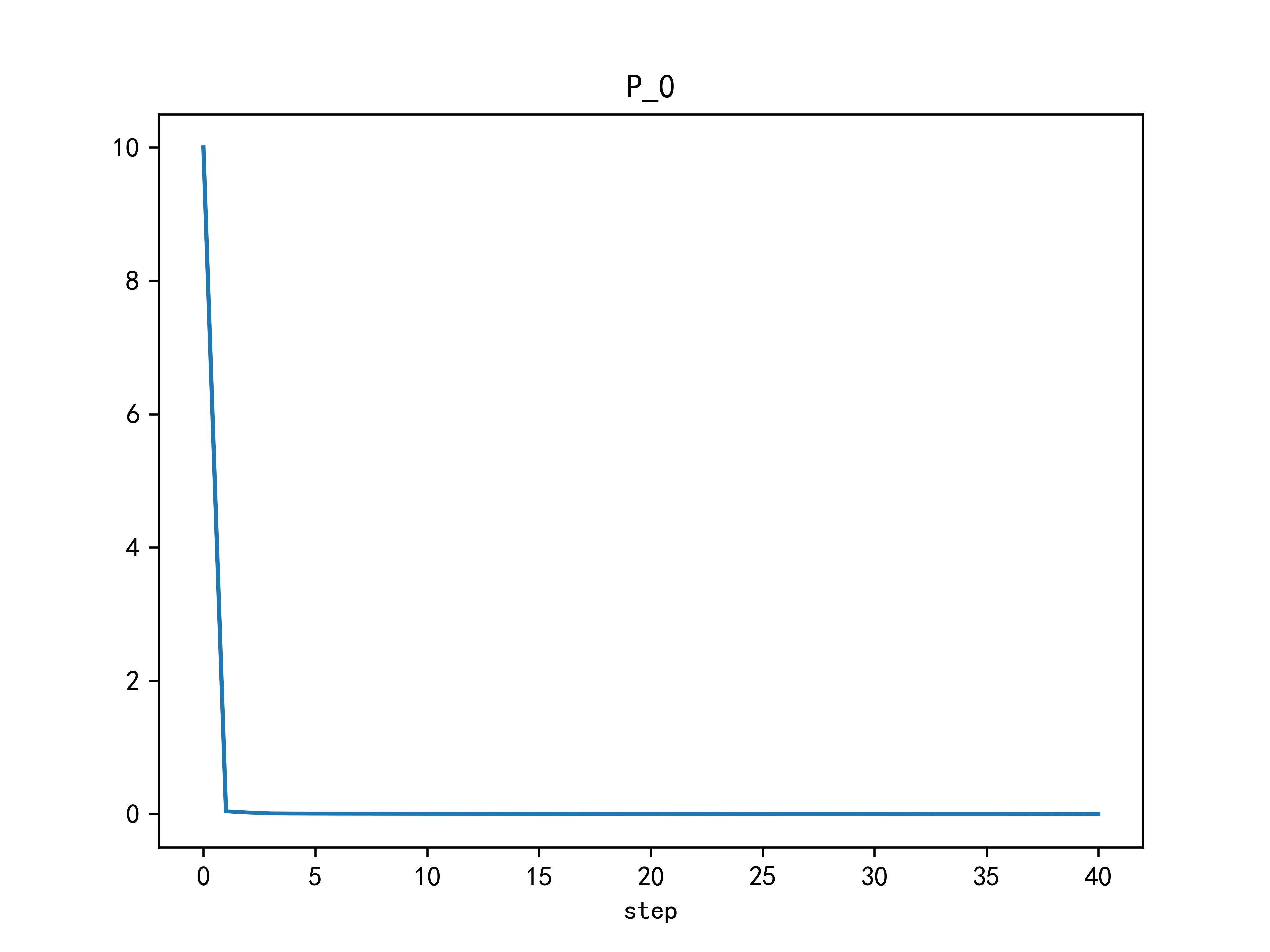
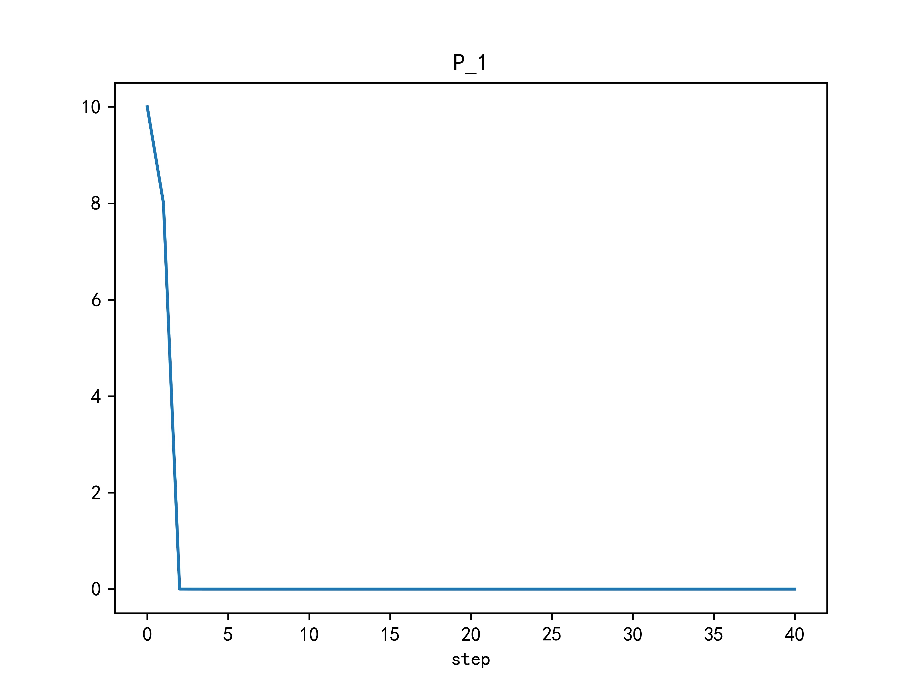
同时,高度和下落速度的估计方差随时间变化为:
|
|
|
|
|
从上图中的结果可以看出,卡尔曼滤波对于物体下落高度和速度的估计在新息一开始加入后就迅速减小,之后渐进减小到0附近之后不再有明显下降。物体自由落体的高度变化曲线为抛物线,速度为匀加速变化,符合自由落体的相关物理定律。
2. 非线性估计问题
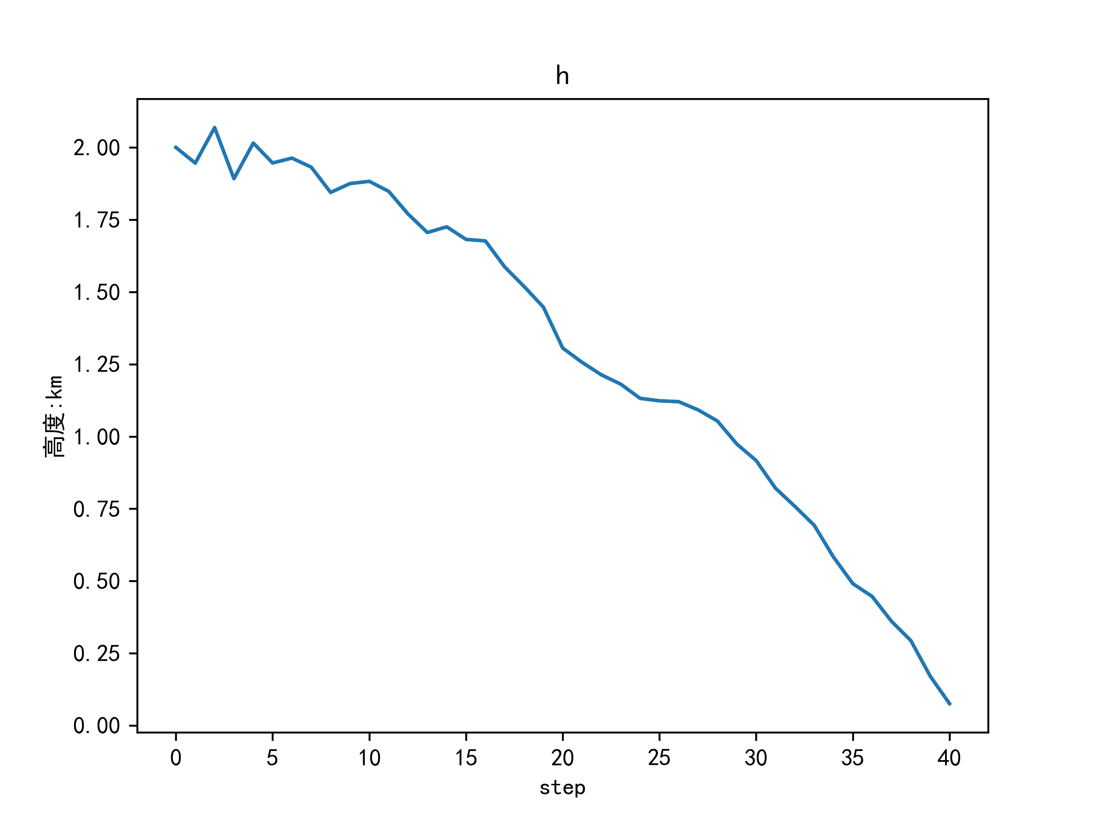
根据题中给出的量测数据以及上文中提到的非线性滤波模型,滤波估计出下落物体的高度和速度变化如下。
物体高度变化为:
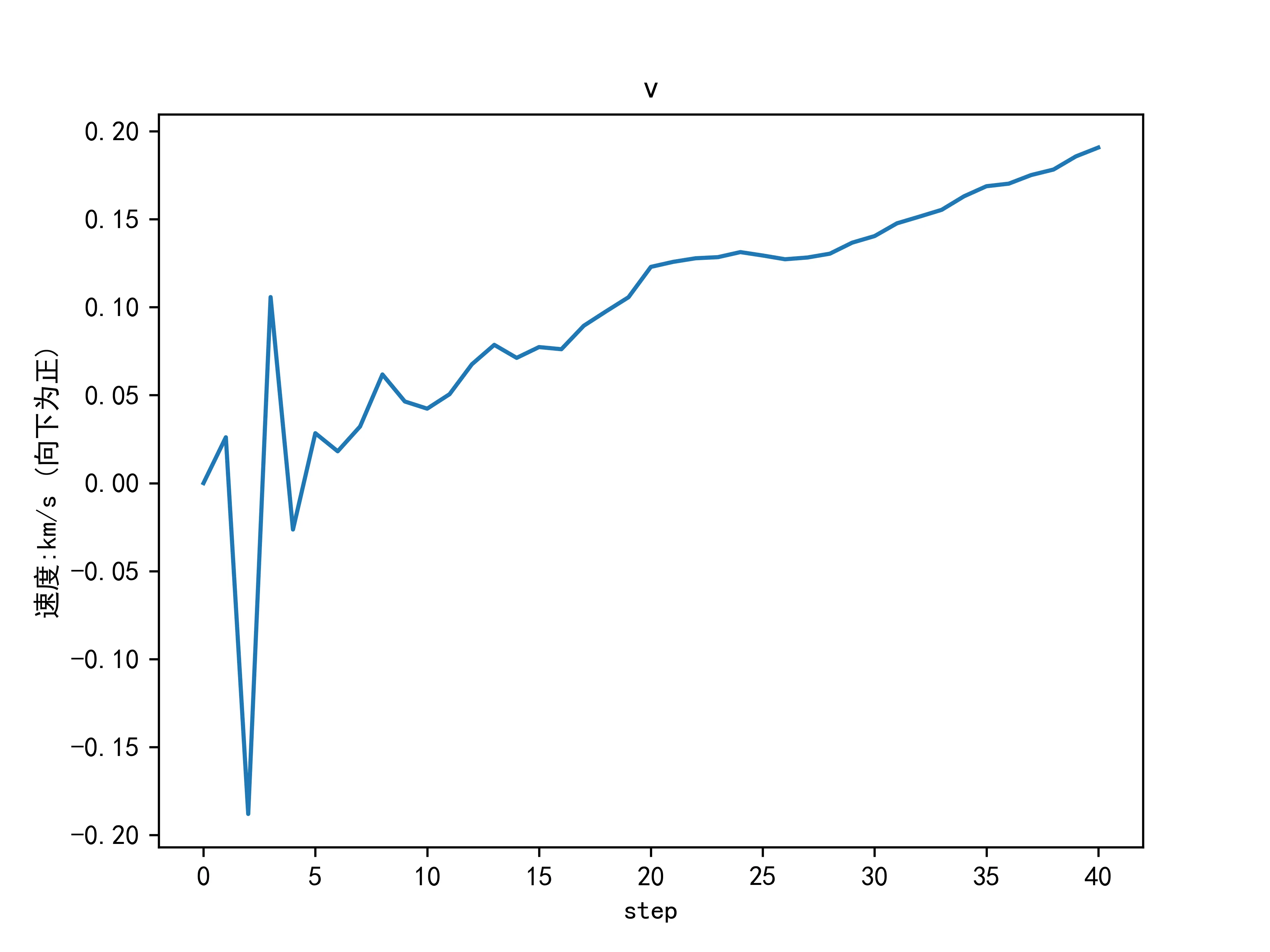
物体下落速度变化为:
物体自由下落高度和速度估计误差为:
|
|
|
|
|
从上图估计结果可以看出,下落高度随时间呈抛物线变化,下落速度(向下为正)随时间匀速上升,符合自由落体物理规律。
实验过程中的一些发现
在最开始的编程和实验过程中,由于题目给出的量测数据以\(km\)为单位,为便于计算,将距离单位统一换算为\(km\)处理。但是由于题面中未给出量测方差的单位,故未对该数值进行换算,即按照单位为\(km\)进行处理。
在求解第1题过程中,未发现任何异常,然而在求解第二题时,如果未对量测协方差进行单位换算,将其单位当作\(km\)进行处理,估计出的结果会如下图所示:
|
|
|
|
|
对比上图中计算结果和实验结果中第二问的计算结果可以看出,相对于线性卡尔曼滤波,非线性卡尔曼滤波在计算时收到量测误差的影响更大。这是由于非线性滤波时量测系数矩阵\(H\)是经过局部线性化得到的,如果量测误差本身较大,则会影响卡尔曼系数的计算结果,最终导致估计结果不准确。
附录
常量配置
1 | ''' |
题目1 代码
1 | ''' |
题目2代码
1 | ''' |